The common narrative in ML is that the MLP layers are effectively a lookup table (see e.g. “Transformer Feed-Forward Layers Are Key-Value Memories”). This is probably a part of the correct explanation but the true story is likely much more complicated. Nevertheless, it would be helpful to understand how NNs represent their mappings in settings where they are forced to memorize, i.e. can’t learn any general features and basically have to build a dictionary.
Most probably a noobish question but I couldn't resist asking.
If a neural network learns either to become a lookup table or to generalize over the data, what would happen if we initialized the weights of the network to be as much as a lookup table as possible?
For example if you have N=1000 data points and only M=100 parameters. Initialize the 100 weights so that each neuron extracts only 1 random data point (without replacement). Could that somehow speedup the training more than starting from pure randomness or gaussian noise?
If then we could also try with initializing a lookup table based on a quick clustering to ensure good representation of the different features from the get go.
What should I know that would make this an obviously stupid idea?
Thanks!
I don't think there is a general answer here. But here are a couple of considerations:
- networks can get stuck in local optima, so if you initialize it to memorize, it might never find a general solution.
- grokking has shown that with high weight regularization, networks can transition from memorized to general solutions, so it is possible to move from one to the other.
- it probably depends a bit on how exactly you initialize the memorized solution. You can represent lookup tables in different ways and some are much more liked by NNs than others. For example, I found that networks really don't like it if you set the weights to one-hot vectors such that one input only maps to one feature.
- My prediction for empirical experiments here would be something like "it might work in some cases but not be clearly better in the general case. It will also depend on a lot of annoying factors like weight decay and learning rate and the exact way you build the dictionary".
Produced as part of the SERI ML Alignment Theory Scholars Program - Winter 2022 Cohort.
I’d like to thank Wes Gurnee, Aryan Bhatt, Eric Purdy and Stefan Heimersheim for discussions and Evan Hubinger, Neel Nanda, Adam Jermyn and Chris Olah for mentorship and feedback.
The post contains a lot of figures, so the suggested length is deceiving. Code can be found in these three colab notebooks [1][2][3].
I have split the post into two parts. The first one is concerned with double descent and other general findings in memorization and the second focuses on measuring memorization using the maximum data dimensionality metric. This is the first post in a series of N posts on memorization in transformers.
Executive summary
I look at a variety of settings and experiments to better understand memorization in toy models. My primary motivation is to increase our general understanding of NNs but I also suspect that understanding memorization better might increase our ability to detect backdoors/trojans.
Isolated components
In the following, we isolate three settings that seem like important components of memorization. They are supposed to model the non-attention parts of a transformer (primarily because I speculate that memorization mostly happens in the non-attention parts).
Bottleneck
By bottleneck we mean a situation in which a model projects from many into fewer dimensions, e.g. from an MLP into the residual stream. We use first use the ReLU output model from the original papers.
X′≈ReLU(WTWx+b)
Replicating work on superposition
We are able to reproduce the main findings of the “basic results” section of the superposition paper. For a model with n=20 data points, m=5 features and an importance distribution of Ii=0.7i, we get basically the same outcomes and plots as in the original paper when sweeping over different sparsities S.
In the following we first plot WTW with corresponding bias terms on the side and then the norms ||Wi|| of the corresponding Ws in the column below. The color corresponds to the superposition metric ∑j(^xixj)2, where yellow means a lot of superposition and black means no superposition and ^xi is x rescaled to unit length.
There is one small caveat, namely that these results seem to be very responsive to the initialization of the bias term. If we don’t initialize it with zeros, the results look significantly different (not shown here; see Adam Jermyn’s work on monosemanticity for possible explanations).
A plausible and unsurprising implication of this finding is that the residual stream (which is much lower dimensional than the embeddings or MLPs) likely contains most or all of its information in superposition. Therefore, probably no feature is important enough to get its own dimension in the residual stream (and there is no reason for features to be in a privileged basis) and we have to look at directions rather than individual dimensions to understand the network.
Replicating work on memorization & double descent
We replicate the double descent phenomenon discussed in the memorization paper. In the paper, they still use the ReLU Output model with m=2 but normalize all inputs. We further adapt this setting in two ways for this post--we use 1000 features instead of 10000 and sparsity 0.99 instead of 0.999. We also cut off the dataset size much earlier than in the original paper. We use the schedulers as described in the paper and can confirm that they make a difference.
Even with these modifications, we can reproduce the double descent phenomenon. The double descent happens exactly 10x earlier than in the original paper which is a result of the 10x smaller features (as indicated by Adam Jermyn’s replication of the original findings). We can also reproduce the progression from memorization to generalization in the columns of W (blue) and hidden activations (red) and the findings on dimensionality as shown below.
We can also plot the fractional dimensionality of the samples and features as described in the paper
We explore the transition between memorization and generalization through the lens of the maximum data dimensionality metric in the second post.
The limits of reconstruction
In the context of transformers, we’re interested in the limits of reconstruction under different conditions. We might think of this roughly as “how much knowledge can the network put into the residual stream?” since the bottleneck setting models a projection from a high-dimensional into a lower-dimensional space.
Thus, we plot the log-loss (MSE) and accuracy for different levels of importance, sparsity, feature sizes and hidden sizes below. To get an approximation of the accuracy, we forward one-hot vectors through the network and measure if the argmax of the output is the same as for the input.[2]
In the first setting, we have noisy inputs with different levels of sparsity and exponentially decreasing importance.[3]
In the second setting, we keep the noise but switch to uniform importance.
And finally, we get rid of the noise and train the network on one-hot vectors.
On the left, we show the results for a setting with exponentially decreasing importance and on the right, we show uniform importance. The fact that the model doesn’t have 100% accuracy in all settings on the right-hand side is likely due to weight decay and other hyperparameters.
Findings from the above figures:
Most of the findings in the previous section seem relatively regular, e.g. the flipping from memorization to generalization during the double descent happens at the same point across different seeds and the effects of dataset size, noise, and importance also seem to follow some pattern. Obviously, this is just a toy setting and the real world is much messier but it makes me slightly more optimistic that we could understand these patterns in real-world networks if we were able to approximate key variables like the noise distribution or the importance of different features.
Furthermore, the number of “facts” we can cram into the residual stream seems to vary a lot between the settings. Under the roughest conditions, i.e. decreasing importance with zero sparsity, the network can only recreate roughly as many one-hot vectors as it has neurons. In the noiseless and uniform setting, on the other hand, it can store a practically unbounded number of concepts. Thus, if real-world text turns out to be fairly sparse, we should expect even small LLMs like GPT2-small to be able to store millions of concepts in superposition in the residual stream (Conjecture's recent post on engineering monosemanticity supports this hypothesis).
The reason this would be interesting for alignment and interpretability is that it would give us better intuitions for what capacity we should expect a network to have. Maybe it wouldn’t even make sense to search for specific niche concepts in small transformers because it turns out that they, e.g., can only reliably represent 10k different concepts. On the other hand, research on this question might increase capabilities faster than alignment and I’m thus not sure if it is worth researching further.
MLP block
The common narrative in ML is that the MLP layers are effectively a lookup table (see e.g. “Transformer Feed-Forward Layers Are Key-Value Memories”). This is probably a part of the correct explanation but the true story is likely much more complicated. Nevertheless, it would be helpful to understand how NNs represent their mappings in settings where they are forced to memorize, i.e. can’t learn any general features and basically have to build a dictionary.
There are many simple behavioral metrics that suggest when a network is a lookup table, e.g. if the training accuracy is 100% and the test accuracy is 0%, this seems like a strong indicator for memorization. However, if we want to provide mechanistic evidence that a model only memorizes, we effectively have to decompile the dictionary into something human-readable and show that all inputs have a unique one-to-one mapping to their corresponding output. In simple toy models, this is easy but even in slightly more complicated toy models, this turns out to be non-trivial. This gets further complicated by the fact that most NNs tend to do a mix of memorization and generalization.
The first section contains replications of some of the findings of Anthropic’s superposition paper which uses a ReLU hidden model and then we switch to the setting found in real transformers, i.e. a conventional MLP in an auto-encoder setting.
Replicating MLP section from superposition paper
The superposition paper contains a section called “Superposition in a Privileged Basis” in which they switch their setting to the “ReLU hidden model”.
h=ReLU(Wx)
x′ =ReLU(WTh+b)
They train a small model with n=10 inputs, m=5 features and Ii=0.75i importance for varying values of sparsity and can show that increasing sparsity leads to increasing superposition.
In the first plot, we look at the first weight of the ReLU hidden model (10 inputs, 5 features). In the case of zero sparsity, the network creates five monosemantic features that we can see in the weights. The more we increase sparsity, the more convoluted the layer becomes. In the second plot, we see the corresponding stack plots (every column in the stack plot represents one column in W) with superposition indications as colors. As we can see, more sparsity implies more polysemanticity.
I can replicate all of the findings, i.e. my results look basically the same as theirs.
While the ReLU hidden layer toy model yields interesting findings on superposition, most real-world networks use a slightly different setting. Therefore, for the rest of the section, we will switch to a standard MLP setting, i.e. two layers with independent weights, two bias terms and one ReLU between the layers but not after the second one.
h=ReLU(W1x+b1)
X′=W2h+b2
For this section we will use an auto-encoder setting, i.e. train with an MSE loss.
In the most simple setting, e.g. orthogonal inputs without noise, we can read the dictionary right off the weights. We can also straightforwardly understand the role of the bias terms (see appendix for both).
Does it show double descent?
Once again, we are interested in whether the MLP setting shows something equivalent to the double descent setting from the bottleneck section.
We find that the MLP shows double descent. Here, the accuracy is defined as 1 if the argmax of the input match the argmax of the output and 0 otherwise. The hidden vectors are defined as Wx+b.
We can also look at the features and hidden vectors after the ReLU.
And before the ReLU.
Furthermore, we find a very similar pattern for the dimensionality of features and datapoints as in the experiments for the output ReLU model.
The horseshoe shapes around the transition between memorization and generalization can be understood as a circle moved by the bias term into the first quadrant. Since the ReLU kills all negative components, the bias term lifts the features into a more positive direction. We can see this by looking at the pre-bias activations (orange) which are not always positive and the bias (purple) which is always positive. This suggests that the ReLU network is doing something roughly similar to the ReLU output model but has to use the bias to shift most computations into the first quadrant.
Given that this adds complexity, we would expect a ReLU model to be worse at memorization but since it has a non-linearity, it can represent much more complicated features.
The rectangles around the origin in the early feature plots above are a result of weight initialization. For small dataset sizes some inputs are never used and the weights are thus not updated. The standard initialization in PyTorch is uniform which looks like a rectangle in 2D. If we change it to Gaussian initialization, the rectangles become circles.
We can also investigate the test loss and accuracy for different values of hidden size and dataset size. The double descent phenomenon seems to happen in all dimensions in a very similar fashion to the original paper, i.e. with increasing dataset size there is a transition region that happens across multiple hidden sizes. Furthermore, we see that the network learns features after the transition since the test accuracy is beyond random guessing level.
Limits of reconstruction
So far, we have primarily looked at settings where the feature size was bigger than the hidden size. However, in transformers, the MLP blocks are usually much bigger than the residual stream. Thus, we care more about the limitations of how much information the MLPs can reconstruct or use from the residual stream.
To test this hypothesis, we use two settings with similar setups. In both cases, we use a random matrix E to project a high-dimensional input into a smaller bottleneck (like a residual stream) and then use an MLP to reconstruct the original input. We use the same setting as in the previous sections, i.e. a fixed dataset of 1000 with a sparsity of 0.99 and varying number of features.
The difference between the two settings (called big fish and small fish due to their shapes in the figure) is what the networks are supposed to reconstruct. In the big fish setting (which was inspired by Adam Jermyn’s work on monosemanticity; it’s called feature decoder there; it’s also related to Conjectures work on monosemanticity), the network is supposed to reconstruct the original input X, in the small fish setting, the network is supposed to learn the identity and reconstruct X’. Intuitively, the big fish setting measures something like “how many facts can we reconstruct from a previous MLP and then project back into a bigger residual stream” and the small fish setting measures something like “how many facts from the residual stream can be used as keys for the look-up table and be projected back” where the dictionary is the identity in this case.
E is a randomly drawn (standard Gaussian) matrix that is supposed to model an embedding. Standard Gaussian matrices have almost always the maximal possible rank, i.e. the size of the bottleneck in our case.
In the following, we will vary the feature size for the two different settings, starting with the big fish setting.
The clearest finding, in this case, is that the bottleneck size does not seem to affect the outcome by a lot and only the hidden size of the network is relevant for its reconstruction loss and accuracy. This suggests that the network is unable to reverse the random matrix projection unless it is given roughly as many dimensions as there are features in the input. It also further reinforces the idea that we can pack a lot of features into a relatively small space (i.e. the bottleneck) using superposition.
We repeat the same setup for the small fish ReLU model.
In this case, we can recover more inputs from the input to the network than in the previous setting. This suggests that computing the identity for superimposed vectors is an easier task for a ReLU network than reverting a random matrix projection (as in the big fish setting). However, the fact that it is still unable to reconstruct all inputs seems to imply that ReLU networks struggle with computations in superposition much more than networks without a ReLU between the layers (which is consistent with our previous findings).
Lastly, we investigate a variant of the small fish setting where we don’t reconstruct X’ (Credit to Chris Olah for suggesting this setup; it’s called re-projector in Adam’s paper). Instead, we create a new random matrix E’ that maps X to X”. Then we force the network to reconstruct X” from X’. Mathematically, we investigate how well an MLP can map from one low-rank representation into another. Intuitively, it encourages to recover true features because it can’t learn the identity. The accuracy is computed by projecting one-hot vectors I through E (resulting in I’) and through E’ (resulting in I”). Then, we forward I’ through the network and compare if the argmax of X” is similar to the argmax of I”.
These results look pretty similar to the big fish setting (confirming Adam Jermyn’s findings). A simple explanation for that would be that in both cases we force the MLP to actually do a computation (translating from a low-rank space into a different space). Given that the amount of information that can be reconstructed is limited primarily by the number of neurons (i.e. hidden size), it seems plausible that the size of the output space doesn’t make a large difference for the ability to reconstruct the input.
Final layer
The unembedding layer in a transformer maps the activations from the residual stream to the tokens in its vocabulary. In some sense, this is similar to the bottleneck setting where we compress a higher dimensional space into a lower dimensional space (e.g. the MLPs that write in the residual stream) and then back into a high-dimensional space (since the size of the vocabulary is usually bigger than the width of the residual stream).
The main difference between the bottleneck settings within the network and in the final layer is the loss function. In the linear layers, we used the MSE loss to approximate the real setting but in the final layer we should use the cross-entropy since that is the correct loss function in most transformers.
In the appendix, we show that networks in the simplest setting are straightforwardly interpretable, i.e. we can read the dictionary off the weights.
Toy unembedding
We investigate a toy unembedding that is similar to the bottleneck setting with the two differences that we don’t use ReLUs and train with cross-entropy loss instead of MSE. The intuition behind this setup is that the residual stream projects into the vocab space through the unembedding. Given that the CE loss has different inductive biases than the MSE loss, we want to understand the differences.
First, we find that the double descent phenomenon still holds in this setting, i.e. the cross-entropy test loss has a clear second peak and the test accuracy is approximately a mirrored version of the test loss. Secondly, we find that the features that were previously mostly circle shaped are now square-shaped during the transition from memorization to generalization.
We want to mechanistically understand how the network memorizes and where the square shape comes from. To this end, we investigate the N=500 setting where the square is most prominent.
In this particular setting, we use hard labels, i.e. the argmax of the input gets converted to the correct class. To ensure that the squares are not a result of hard labels, we test the same setting with soft labels, i.e. by using the input as the target. We find the same squares (see appendix). Furthermore, we also verify that using W1 and W2 instead of W and WT is not the root of the squares (see appendix).
To understand where the squares come from we can mechanistically interpret how the network memorizes the inputs. We start by observing that W1 has a square shape, the hidden vectors have a sort of rose shape and W2 is a circle.
To get the logit for any input we compute the inner product of the hidden vectors and W2 and then add the respective bias term (i.e. Whi+b). To understand how the network maps the hidden vectors to the correct logits, we split this step up into parts. We pick the first three hidden vectors and multiply them with W2 respectively.
The result can be seen as a rotation, stretching and scaling of W2 by hi. The values colored in black denote the term that corresponds to the maximum of the inputs. Note that the black dots are all in the first quadrant because there both vector entries are positive.
Now we complete the second step of the logit computation, i.e. summing both components and adding the bias. This can be seen as projecting the circle into one dimension.
After that projection, we find that the output that corresponds to the correct class always ends up on top of all others after the bias was added. In the presented examples, the bias actually reduces the maximum but there are opposite examples as well (not shown). Importantly, since this setting includes hard labels, we only care about the position of the maximum.
Thus, we now understand the second part of the algorithm. The rose-shaped hidden activations rotate, stretch and scale the circle of W2 into a position where the correct entry is in the first quadrant. Then the sum of both components and the bias ensure that the correct value is in fact the maximum of the outputs.
Now the second question is why do we need the rectangle to create this particular hidden pattern from the inputs. In our setting, S=0.99, F=1000 and D=500 which means there are 10 active features per datapoint on average and there are fewer datapoints than features. Thus, the model likely doesn’t learn any general features and just memorizes the data. Since the network has 100% training accuracy and 0% test accuracy, this seems very plausible. However, since we have 500 datapoints, some of them likely share features with each other.
Thus, the task of W1 boils down to “find a structure in 2D which allows you to map a 1000-dimensional input with roughly 10 non-zero uniformly distributed features into the required rose shape”. I have not fully understood why a rectangle is the best shape for this task but empirically the network seems to perform some sort of weighted vote to choose the position of the hidden vectors. Intuitively, it chooses the ratio of quadrants by taking a weighted vote between the corners of the square and adapt the position with points in the middle. My guess would be that the square shape makes it easier to balance uniformly distributed features across datapoints but I have no mathematical argument for this.
Importantly, the square is not a consequence if a uniform initialization of W1. The same pattern also emerges when we use Xavier initialization, i.e. normally distributed weights.
While it felt rewarding to understand the exact mechanism by which this network memorizes, unfortunately, there is not a lot of general insight from this example. This particular setting seems to be a special case and we don’t expect it to hold in real-world models. Furthermore, it doesn’t feel like we have gained that much meaningful insight into transformers which is why we will focus on small toy transformers in the next part of the series.
Intermediate conclusions
My main takeaways from this research are
Appendix
Linear block
In the following, we see that we can easily read the weights and activations of small MLPs that memorize orthogonal data.
Noiseless setting - orthogonal inputs
To understand the basic case of what an MLP is doing when we force it to memorize we consider a setting where we have n=20 orthogonal inputs and m=10 neurons. We use a noiseless setting and use one-hot vectors as data. Thus, the network is supposed to memorize the identity.
In this case, the algorithm can be easily read off the weights, i.e. it is a dictionary where each weight corresponds to an activation. It really is just a sequence of two key-value pairs.
In this simple toy setting, we can investigate the role of the first bias term. We can see that the first bias “counters” the ReLU in the sense that it lifts all activations before it barely above 0.
The role of the second bias term is a bit more nebulous. Intuitively, it acts as an “equalizer”, i.e. it adds constants to the logits such that they are more evenly distributed which is favored by the cross-entropy loss. However, the weights of the second bias term seems to be, to a large extent, due to the initialization of weights in W2 (not shown here).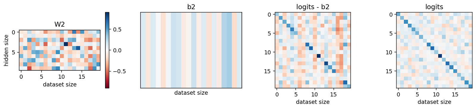
When we compare the hidden size vs. dataset size scaling for orthogonal noiseless inputs (i.e. one-hot vectors), we see that an MLP trained with MSE struggles to accurately reconstruct the input when the hidden size is much lower than the dataset size. In the cases without ReLUs in the middle, we did not have this problem and it seems to suggest that the ReLU makes superposition harder.
Misc
Cosine similarities for different combinations of data and hidden size. We find that the cosine similarities cluster around a certain range of values for some cases. Intuitively this would mean that they all have the same angle to each other which would make sense in the case of memorization. However, for other samples, the distribution is all over the place which makes me think that the cosine similarity, as applied here, basically tells us very little about memorization.
MLP double descent but with the second ReLU term.
The squares still show up, so they are not an artifact of leaving out the ReLU term. By now we know that they come from the initialization, so this finding is not surprising.
Final layer
Ignoring the residual stream for a second
Let’s ignore the fact that there is a residual stream for a second and pretend that the outgoing layer of the final MLP directly connects to the unembedding. Without a layer norm, we can combine the final linear layer and the unembedding to one big matrix connecting neurons to logits.
Usually this setting “opens up”, i.e. the vocab size is larger than the width of the final MLP (just barely true for GPT-3, might soon not be true anymore). Thus, we first try to understand such a setting in an MLP with a hidden size of 2 and 64 unique one-hot vectors as inputs.
We find that the first set of weights projects inputs in all directions but the bias “lifts” them above 0 and thus into the first quadrant such that they don’t get killed by the ReLU. The activations span nearly the entire 90-degree angle that they can use. Furthermore, activation vectors that are close to each other (i.e. have similar angles) tend to have different lengths. I suspect that makes it less likely that W2 confuses them for the same input. These activations then get multiplied with W2 and the bias makes sure that the correct value is selected (more details on this mechanism in the next section).
We now switch to a familiar toy setting and look at an MLP with n=20 inputs and m=10 neurons. Once again, we can read the algorithm/dictionary off the weights. In the first setting, we train for 1000 epochs and in the second for 3000.
We can observe a couple of things here. First, MLPs trained with cross-entropy loss (and low weight decay) love big activations and strongly negative weights in W2. The intuition here is that cross-entropy wants to make the correct logit go to +inf and all others to -inf (if we train for long enough). Since it is harder to increase one logit than to decrease N-1 others, the incentive is to make W2 negative. Secondly, this shows that a naive application of the cosine similarity on the activations is not a good detector of memorization. This network has perfectly memorized the training data and yet the cosine similarities of the activations are very close to 1 (at least in the second case).
The biases take similar roles as in the MSE setting, i.e. the first bias term lifts all the activations above 0 and the second bias term balances the logits.
Weight decay also plays a predictable role in this setting, i.e. a weight decay of 1 counteracts the desired of cross-entropy to make everything go to infinity. This mostly shows that cross-entropy has a different inductive bias than MSE and also that weight decay can lead to more easily interpretable results (at least in this setting).
When we train the network on antipodal one-hot vectors (e.g. [1,0,...] -> 0, [-1,0,...] -> 1, etc.) the model effectively uses half of the weights for one input and the other half for the opposite input and these parts do not interact with each other.
In this case, we can still read the dictionary off the weights. However, we can already see that this will be hard or impossible in more complicated settings where the inputs are not orthogonal, etc.
When we look at the dataset size vs. hidden size scaling for MLPs trained with CE, we see that small hidden sizes do not pose any meaningful limit for reconstruction loss (white squares indicate 0 loss) or accuracy. This is possibly due to the fact that the cross entropy only requires creating an output that is bigger than all others while the MSE requires recreating absolute values.
Intuitively, these results say something like “if the residual stream has many concepts in superposition, the unembedding will almost surely be able to decode them (modulo noise)” or in other words, the unembedding is unlikely to be a bottleneck for how many different concepts a transformer can learn.
More findings on double descent
Comparison to soft labels. Shows the squares again, so it’s not an artifact of hard labels.
Double descent in the original setting with W1 and W2 instead of W, W.T. Also finds circles, so the squares don’t come from splitting W1 and W2.
Misc
When we use the cross-entropy loss, the cosine similarities are just always 1 if the weight decay is not high enough. This means that a naive application of the cosine similarity tells us not that many relevant things about memorization or at least we have to be careful with the setting.
This work would pretty straightforwardly lead to capability gains, so I’m not sure it’s worth pursuing.
Note that importance is not factored into the accuracy but is factored into the log-loss.
The rule is: 100 ** -torch.linspace(0, 1, feature_size)