The easiest way to explain why this is the case will probably be to provide an example. Suppose we have a Bayesian learning machine with 15 parameters, whose parameter-function map is given by
and whose loss function is the KL divergence. This learning machine will learn 4-degree polynomials. Moreover, it is overparameterised, and its loss function is analytic in its parameters, etc, so SLT will apply to it.
In your example there are many values of the parameters that encode the zero function (e.g. and all other parameters free) in addition to there being many parameters that encode the function (e.g. , variables free and ). Without thinking about it more I'm not sure which is actually has local learning coefficient (RLCT) and therefore counts as "more simple" from an SLT perspective.
However, if I understand correctly it's not this specific example that you care about. We can agree that there is some way of coming up with a simple model which (a) can represent both the functions and and (b) has parameters and respectively representing these functions with local learning coefficients . That is, according to the local learning coefficient as a measure of model complexity, the neighbourhood of the parameter is more complex than that of . I believe your observation is that this contradicts an a priori notion of complexity that you hold about these functions.
Is that a fair characterisation of the argument you want to make?
Assuming it is, my response is as follows. I'm guessing you think is simpler than because the former function can be encoded by a shorter code on a UTM than the latter. But this isn't the kind of complexity that SLT talks about: the local learning coefficient that appears in the main theorems represents the complexity of representing a given probability distribution using parameters from the model, and is not some intrinsic model-free complexity of the distribution itself.
One way of saying it is that Kolmogorov complexity is the entropy cost of specifying a machine on the description tape of a UTM (a kind of absolute measure) whereas the local learning coefficient is the entropy cost per sample of incrementally refining an almost true parameter in the neural network parameter space (a kind of relative measure). I believe they're related but not the same notion, as the latter refers fundamentally to a search process that is missing in the former.
We can certainly imagine a learning machine set up in such a way that it is prohibitively expensive to refine an almost true parameter nearby a solution that looks like and very cheap to refine an almost true parameter near a solution like , despite that being against our natural inclination to think of the former as simpler. It's about the nature of the refinement / search process, not directly about the intrinsic complexity of the functions.
So we agree that Kolmogorov complexity and the local learning coefficient are potentially measuring different things. I want to dig deeper into where our disagreement lies, but I think I'll just post this as-is and make sure I'm not confused about your views up to this point.
suppose we have a 500,000-degree polynomial, and that we fit this to 50,000 data points. In this case, we have 450,000 degrees of freedom, and we should by default expect to end up with a function which generalises very poorly. But when we train a neural network with 500,000 parameters on 50,000 MNIST images, we end up with a neural network that generalises well. Moreover, adding more parameters to the neural network will typically make generalisation better, whereas adding more parameters to the polynomial is likely to make generalisation worse.
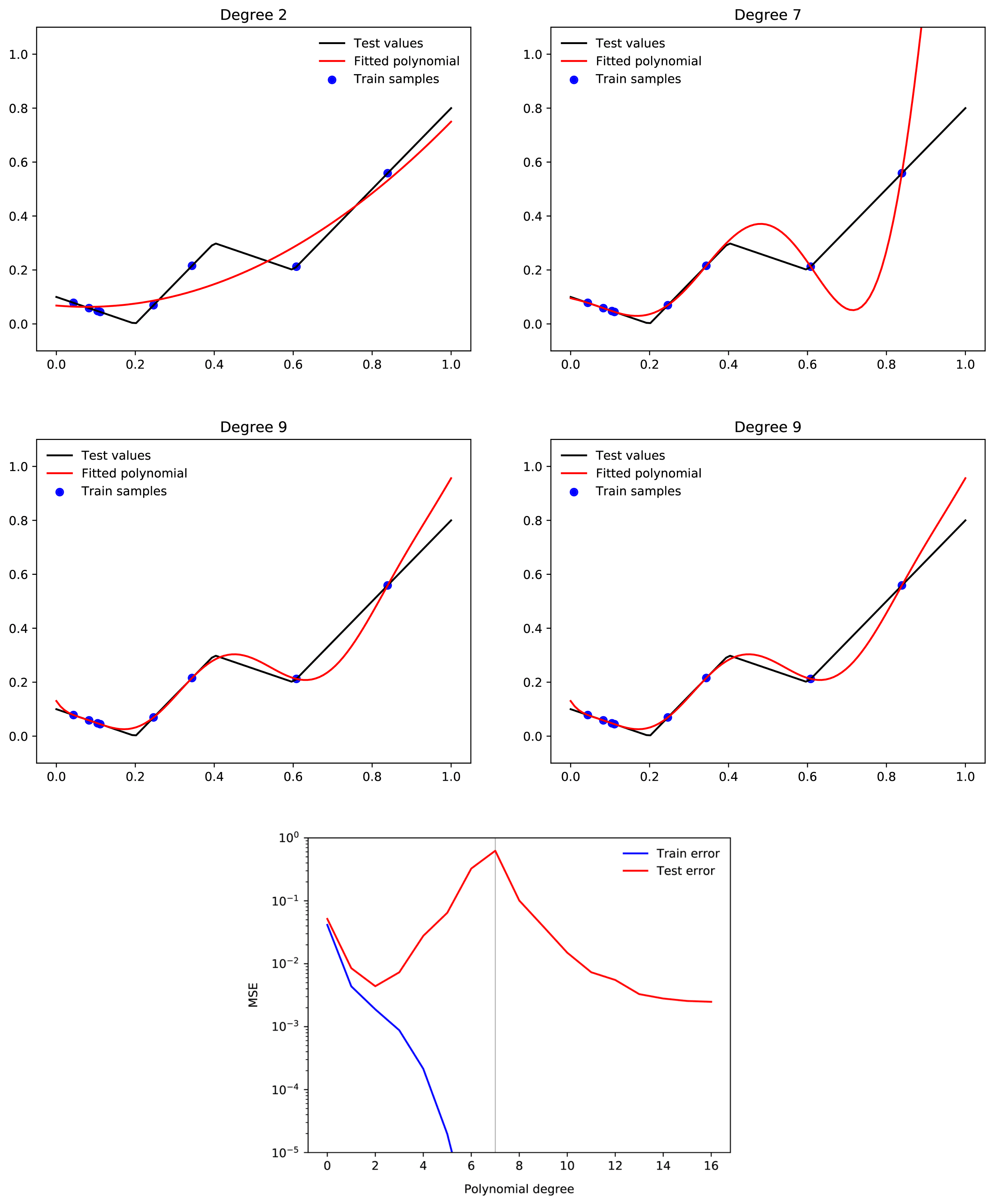
Only tangentially related, but your intuition about polynomial regression is not quite correct. A large range of polynomial regression learning tasks will display double descent where adding more and more higher degree polynomials consistently improves loss past the interpolation threshold.
Examples from here:
Relevant paper
I think I agree that SLT doesn't offer an explanation of why NNs have a strong simplicity bias, but I don't think you have provided an explanation for this either?
Here's a simple story for why neural networks have a bias to functions with low complexity (I think it's just spelling out in more detail your proposed explanation):
Since the Kolmogorov complexity of a function is (up to a constant offset) equal to the minimum description length of the function, it is upper bounded by any particular way of describing the function, including by first specifying a parameter-function map, and then specifying the region of parameter space corresponding to the function. That means:
where is the minimum description length of the parameter function map, is the minimum description length required to specify given , and the term comes from the fact that K complexity is only defined up to switching between UTMs. Specifying given entails specifying the region of parameter space corresponding to defined by Since we can use each bit in our description of to divide the parameter space in half, we can upper bound the mdl of given by [1] where denotes the size of the overall parameter space. This means that, at least asymptotically in , we arrive at
This is (roughly) a hand-wavey version of the Levin Coding Theorem (a good discussion can be found here). If we assume a uniform prior over parameter space, then . In words, this means that the prior assigned by the parameter function map to complex functions must be small. Now, the average probability assigned to each function in the set of possible outputs of the map is where is the number of functions. Since there are functions with K complexity at most , the highest K complexity of any function in the model must be at least so, for simple parameter function maps, the most complex function in the model class must be assigned prior probability less than or equal to the average prior. Therefore if the parameter function map assigns different probabilities to different functions, at all, it must be biased against complex functions (modulo the term)!
But, this story doesn't pick out deep neural network architectures as better parameter function maps than any other. So what would make a parameter function map bad? Well, for a start the term includes — we can always choose a pathologically complicated parameter function map which specifically chooses some specific highly complex functions to be given a large prior by design. But even ignoring that, there are still low complexity maps that have very poor generalisation, for example polyfits. That's because the expression we derived is only an upper bound: there is no guarantee that this bound should be tight for any particular choice of parameter-function map. Indeed, for a wide range of real parameter function maps, the tightness of this bound can vary dramatically:
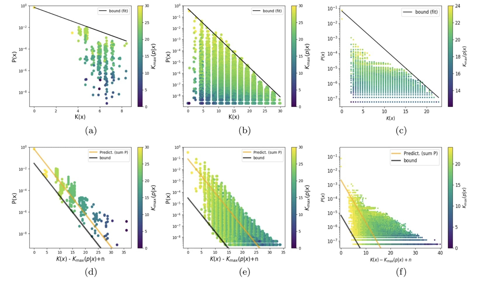
This figure (from here) shows scatter plots of (an upper bound estimate of) the K complexity of a large set of functions, against the prior assigned to them by a particular choice of param function map.
It seems then that the question of why neural network architectures have a good simplicity bias compared to other architectures is not about why they do not assign high volume/prior to extremely complicated functions — since this is satisfied by all simple parameter function maps — but why there are not many simple functions that they do not assign high prior to relative to other parameter-function maps — why the bottom left of these plots is less densely occupied, or occupied with less 'useful' functions, for NN architectures than other architectures. Of course, we know that there are simple functions that the NN inductive bias hates (for example simple functions with a for loop cannot be expressed easily by a feed forward NN), but we'd like to explain why they have fewer 'blind spots' than other architectures. Your proposed solution doesn't address this part of the question I think?
Where SLT fits in is to provide a tool for quantifying for any particular . That is, SLT provides a sort of 'cause' for how different functions occupy regions of parameter space of different sizes: namely that the size of can be measured by counting a sort of effective number of parameters present in a particular choice [2]. Put another way, SLT says that if you specify by using each bit in your description to cut in half, then it will sort-of take bits (the local learning coefficient at the most singular point in parameter space that maps to ) to describe , so for some constant that is independent of .
So your explanation says that any parameter function map is biased to low complexity functions, and SLT contributes a way to estimate the size of the parameter space assigned to a particular function, but neither addresses the question of why neural networks have a simplicity bias that is stronger than other parameter function maps.
- ^
Actually, I am pretty unsure how to do this properly. It seems like the number of bits required to specify that a point is inside some region in a space really ought to depend only on the fraction of the space occupied by the region, but I don't know how to ensure this in general - I'd be keen to know how to do this. For example, if I have a 2d parameter space (bounded, so a large square), and is a random square, is a union of 100 randomly placed squares, does it take the same number of bits to find my way into either (remember, I don't need to fully describe the region, just specify that I am inside it)? Or even more simply, if is the set of points within distance of the line , I can specify I am within the region by specifying the coordinate up to resolution , so . If is the set of points within distance of the line , how do I specify that I am within in a number of bits that is asymptotically equal to as ?
- ^
In fact, we might want to say that at some imperfect resolution/finite number of datapoints, we want to treat a set of very similar functions as the same, and then the best point in parameter space to count effective parameters at is a point that maps to the function which gets the lowest loss in the limit of infinite data.
One argument sketch using SLT that NNs are biased towards low complexity solutions: suppose reality is generated by a width 3 network, and you're modelling it with a width 4 network. Then, along with the generic symmetries, optional solutions also have continuous symmetries where you can switch which neuron is turned off.
Roughly, say neurons 3 and 4 have the same input weight vectors (so their activations are the same), but neuron 4's output weight vector is all zeros. Then you can continuously scale up the output vector of neuron 4 while simultaneously scaling down the output vector of neuron 3 to leave the network computing the same function. Also, when neuron 4 has zero weights as inputs and outputs you can arbitrarily change the inputs or the outputs but not both.
Anyway, this means that when the data is generated by a slim neural net, optimal nets will have a good RLCT, but when it's generated by a neural net of the right width, optimal nets will have a bad RLCT. So nets can learn simple data, and it's easier for them to learn simple data than complex data - assuming thin neural nets count as simple.
This is basically a justification of something like your point 1, but AFAICT it's closer to a proof in the SLT setting than in your setting.
Does this not essentially amount to just assuming that the inductive bias of neural networks in fact matches the prior that we (as humans) have about the world?
This is basically a justification of something like your point 1, but AFAICT it's closer to a proof in the SLT setting than in your setting.
I think it could probably be turned into a proof in either setting, at least if we are allowed to help ourselves to assumptions like "the ground truth function is generated by a small neural net" and "learning is done in a Bayesian way", etc.
Does this not essentially amount to just assuming that the inductive bias of neural networks in fact matches the prior that we (as humans) have about the world?
No? It amounts to assuming that smaller neural networks are a better match for the actual data generating process of the world.
The assumption that small neural networks are a good match for the actual data generating process of the world, is equivalent to the assumption that neural networks have an inductive bias that gives large weight to the actual data generating process of the world, if we also append the claim that neural networks have an inductive bias that gives large weight to functions which can be described by small neural networks (and this latter claim is not too difficult to justify, I think).
The easiest way to explain why this is the case will probably be to provide an example. Suppose we have a Bayesian learning machine with 15 parameters, whose parameter-function map is given by
and whose loss function is the KL divergence. This learning machine will learn 4-degree polynomials.
I'm not sure, but I think this example is pathological. One possible reason for this to be the case is that the symmetries in this model are entirely "generic" or "global." The more interesting kinds of symmetry are "nongeneric" or "local."
What I mean by "global" is that each point in the parameter space has the same set of symmetries (specifically, the product of a bunch of hyperboloids ). In neural networks there are additional symmetries that are only present for a subset of the weights. My favorite example of this is the decision boundary annihilation (see below).
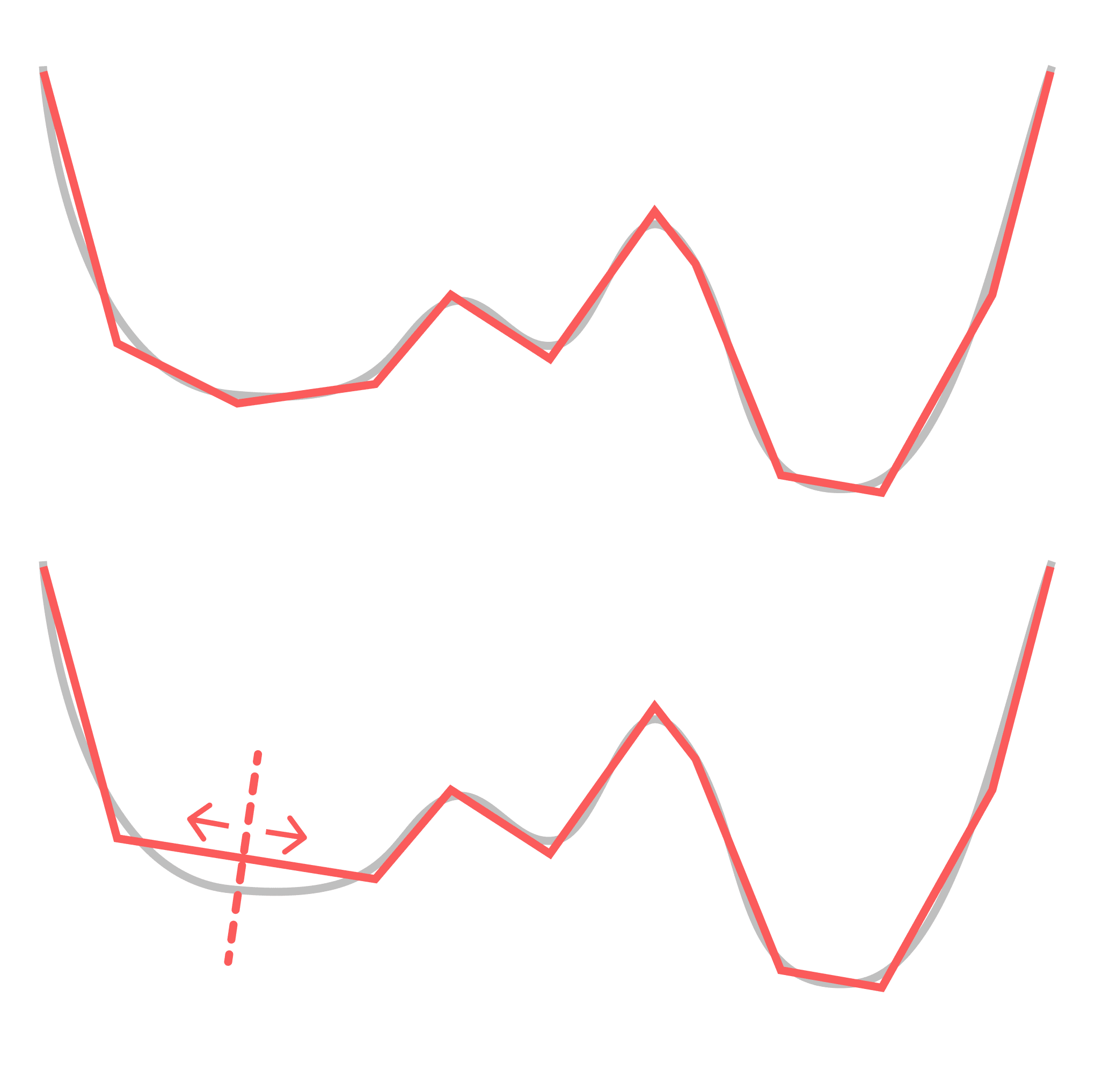
For the sake of simplicity, consider a ReLU network learning a 1D function (which is just piecewise linear approximation). Consider what happens when you you rotate two adjacent pieces so they end up sitting on the same line, thereby "annihilating" the decision boundary between them, so this now-hidden decision boundary no longer contributes to your function. You can move this decision boundary along the composite linear piece without changing the learned function, but this only holds until you reach the next decision boundary over. I.e.: this symmetry is local. (Note that real-world networks actually seem to take advantage of this property.)
This is the more relevant and interesting kind of symmetry, and it's easier to see what this kind of symmetry has to do with functional simplicity: simpler functions have more local degeneracies. We expect this to be true much more generally — that algorithmic primitives like conditional statements, for loops, composition, etc. have clear geometric traces in the loss landscape.
So what we're really interested in is something more like the relative RLCT (to the model class's maximum RLCT). This is also the relevant quantity from a dynamical perspective: it's relative loss and complexity that dictate transitions, not absolute loss or complexity.
This gets at another point you raised:
2. It is a type error to describe a function as having low RLCT. A given function may have a high RLCT or a low RLCT, depending on the architecture of the learning machine.
You can make the same critique of Kolmogorov complexity. Kolmogorov complexity is defined relative to some base UTM. Fixing a UTM lets you set an arbitrary constant correction. What's really interesting is the relative Kolmogorov complexity.
In the case of NNs, the model class is akin to your UTM, and, as you show, you can engineer the model class (by setting generic symmetries) to achieve any constant correction to the model complexity. But those constant corrections are not the interesting bit. The interesting bit is the question of relative complexities. I expect that you can make a statement similar to the equivalence-up-to-a-constant of Kolmogorov complexity for RLCTs. Wild conjecture: given two model classes and and some true distribution , their RLCTs obey:
where is some monotonic function.
I'm not sure, but I think this example is pathological.
Yes, it's artificial and cherry-picked to make a certain rhetorical point as simply as possible.
This is the more relevant and interesting kind of symmetry, and it's easier to see what this kind of symmetry has to do with functional simplicity: simpler functions have more local degeneracies.¨
This is probably true for neural networks in particular, but mathematically speaking, it completely depends on how you parameterise the functions. You can create a parameterisation in which this is not true.
You can make the same critique of Kolmogorov complexity.
Yes, I have been using "Kolmogorov complexity" in a somewhat loose way here.
Wild conjecture: [...]
Is this not satisfied trivially due to the fact that the RLCT has a certain maximum and minimum value within each model class? (If we stick to the assumption that is compact, etc.)
This is probably true for neural networks in particular, but mathematically speaking, it completely depends on how you parameterise the functions. You can create a parameterisation in which this is not true.
Agreed. So maybe what I'm actually trying to get at it is a statement about what "universality" means in the context of neural networks. Just as the microscopic details of physical theories don't matter much to their macroscopic properties in the vicinity of critical points ("universality" in statistical physics), just as the microscopic details of random matrices don't seem to matter for their bulk and edge statistics ("universality" in random matrix theory), many of the particular choices of neural network architecture doesn't seem to matter for learned representations ("universality" in DL).
What physics and random matrix theory tell us is that a given system's universality class is determined by its symmetries. (This starts to get at why we SLT enthusiasts are so obsessed with neural network symmetries.) In the case of learning machines, those symmetries are fixed by the parameter-function map, so I totally agree that you need to understand the parameter-function map.
However, focusing on symmetries is already a pretty major restriction. If a universality statement like the above holds for neural networks, it would tell us that most of the details of the parameter-function map are irrelevant.
There's another important observation, which is that neural network symmetries leave geometric traces. Even if the RLCT on its own does not "solve" generalization, the SLT-inspired geometric perspective might still hold the answer: it should be possible to distinguish neural networks from the polynomial example you provided by understanding the geometry of the loss landscape. The ambitious statement here might be that all the relevant information you might care about (in terms of understanding universality) are already contained in the loss landscape.
If that's the case, my concern about focusing on the parameter-function map is that it would pose a distraction. It could miss the forest for the trees if you're trying to understand the structure that develops and phenomena like generalization. I expect the more fruitful perspective to remain anchored in geometry.
Is this not satisfied trivially due to the fact that the RLCT has a certain maximum and minimum value within each model class? (If we stick to the assumption that is compact, etc.)
Hmm, maybe restrict so it has to range over .
If a universality statement like the above holds for neural networks, it would tell us that most of the details of the parameter-function map are irrelevant.
I suppose this depends on what you mean by "most". DNNs and CNNs have noticeable and meaningful differences in their (macroscopic) generalisation behaviour, and these differences are due to their parameter-function map. This is also true of LSTMs vs transformers, and so on. I think it's fairly likely that these kinds of differences could have a large impact on the probability that a given type of model will learn to exhibit goal-directed behaviour in a given training setup, for example.
The ambitious statement here might be that all the relevant information you might care about (in terms of understanding universality) are already contained in the loss landscape.
Do you mean the loss landscape in the limit of infinite data, or the loss landscape for a "small" amount of data? In the former case, the loss landscape determines the parameter-function map over the data distribution. In the latter case, my guess would be that the statement probably is false (though I'm not sure).
EDIT: What I wrote here is wrong; the loss landscape does not determine the parameter-function map even in the limit of infinite data (except if we consider a binary classification problem without noise, and consider the loss for each parameter assignment and input with support under the data distribution).
In this post, I will briefly give my criticism of Singular Learning Theory (SLT), and explain why I am skeptical of its significance. I will especially focus on the question of generalisation --- I do not believe that SLT offers any explanation of generalisation in neural networks. I will also briefly mention some of my other criticisms of SLT, describe some alternative solutions to the problems that SLT aims to tackle, and describe some related research problems which I would be more excited about.
(I have been meaning to write this for almost 6 months now, since I attended the SLT workshop last June, but things have kept coming in the way.)
For an overview of SLT, see this sequence. This post will also refer to the results described in this post, and will also occasionally touch on VC theory. However, I have tried to make it mostly self-contained.
The Mystery of Generalisation
First of all, what is the mystery of generalisation? The issue is this; neural networks are highly expressive, and typically overparameterised. In particular, when a real-world neural network is trained on a real-world dataset, it is typically the case that this network is able to express many functions which would fit the training data well, but which would generalise poorly. Moreover, among all functions which do fit the training data, there are more functions (by number) that generalise poorly, than functions that generalise well. And yet neural networks will typically find functions that generalise well. Why is this?
To make this point more intuitive, suppose we have a 500,000-degree polynomial, and that we fit this to 50,000 data points. In this case, we have 450,000 degrees of freedom, and we should by default expect to end up with a function which generalises very poorly. But when we train a neural network with 500,000 parameters on 50,000 MNIST images, we end up with a neural network that generalises well. Moreover, adding more parameters to the neural network will typically make generalisation better, whereas adding more parameters to the polynomial is likely to make generalisation worse. Why is this?
A simple hypothesis might be that some of the parameters in a neural network are redundant, so that even if it has 500,000 parameters, the dimensionality of the space of all functions which it can express is still less than 500,000. This is true. However, the magnitude of this effect is too small to solve the puzzle. If you get the MNIST training set, and assign random labels to the test data, and then try to fit the network to this function, you will find that this often can be done. This means that while neural networks have redundant parameters, they are still able to express more functions which generalise poorly, than functions which generalise well. Hence the puzzle.
The anwer to this puzzle must be that neural networks have an inductive bias towards low-complexity functions. That is, among all functions which fit a given training set, neural networks are more likely to find a low-complexity function (and such functions are more likely to generalise well, as per Occam's Razor). The next question is where this inductive bias comes from, and how it works. Understanding this would let us better understand and predict the behaviour of neural networks, which would be very useful for AI alignment.
I should also mention that generalisation only is mysterious when we have an amount of training data that is small relative to the overall expressivity of the learning machine. Classical statistical learning theory already tells us that any sufficiently well-behaved learning machine will generalise well in the limit of infinite training data. For an overview of these results, see this post. Thus, the question is why neural networks can generalise well, given small amounts of training data.
The SLT Answer
SLT proposes a solution to this puzzle, which I will summarise below. This summary will be very rough --- for more detail, see this sequence and this post.
First of all, we can decompose a neural network into the following components:
1. A parameter space, Θ, corresponding to all possible assignments of values to the weights.
2. A function space, F, which contains all functions that the neural network can express.
3. A parameter-function map, m:Θ→F, which associates each parameter assignment θ∈Θ with a function f∈F.
SLT models neural networks (and other learning machines) as Bayesian learners, which have a prior over Θ, and update this prior based on the training data in accordence with Bayes' theorem. Moreover, it also assumes that the loss (ie, the likelihood) of the network is analytic in Θ. This essentially amounts to a kind of smoothness assumption. Moreover, as is typical in the statistical learning theory literature, SLT assumes that the training data (and test data) is drawn i.i.d. from some underlying data distribution (though there are some ways to relax this assumption).
We next observe that a neural network typically is overparameterised, in the sense that there for a particular function f∈F typically will be many different parameter assignments θ∈Θ such that m(θ)=f. For example, we can almost always rescale different parameters without affecting the input-output behaviour of a neural network. There can also be symmetries --- for example, we can always re-shuffle the neurons in a neural network, which would also never affect its input-output behaviour. Finally, there can be redundancies, where some parameters or parts of the network are not used for any piece of training data.
These symmetries and redundancies lead to paths or valleys of constant loss through the loss landscape, which are created by the fact that the parameters θ can be continuously moved in some direction without affecting the function f expressed by the network.
Next, note that if we are in such a valley, then we can think of the neural network as having a local "effective parameter dimension" that is lower than the full dimensionality of Θ. For example, if Θ has 10 dimensions, but there is a (one-dimensional) valley along which m (and hence f, and hence the loss) is constant, then the effective parameter dimension of the network is only 9. Moreover, this "effective parameter dimension" can be different in different regions of Θ; if two one-dimensional valleys intersect, then the effective parameter dimension at that point is only 8, since we can move in two directions without changing f. And so on. SLT proposes a measurement, called the RLCT, which provides a continuous quantification of the "effective parameter dimension" at different points. If a point or region has a lower RLCT, then that means that there are more redundant parameters in that region, and hence that the effective parameter dimension is lower.
SLT provides a theorem which says that, under the assumptions of the theory, points with low RLCT will eventually dominate the Bayesian posterior, in the limit of infinite data. It is worth noting that this theorem does not require any strong assumptions about the Bayesian prior over Θ. This should be reasonably intuitive. Very loosely speaking, regions with a low RLCT have a larger "volume" than regions with high RLCT, and the impact of this fact eventually dominates other relevant factors. (However, this is a very loose intuition, that comes with several caveats. For a more precise treatment, see the posts linked above.)
Moreover, since regions with a low RLCT roughly can be thought of as corresponding to sub-networks with fewer effective parameter dimensions, we can (perhaps) think of these regions as corresponding to functions with low complexity. Putting this together, it seems like SLT says that overparameterised Bayesian learning machines in the limit will pick functions that have a low complexity, and such functions should also generalise well. Indeed, SLT also provides a theorem which says that the Bayes generalisation loss eventually will be low, where the Bayes generalisation loss is a Bayesian formalisation of prediction error. So this solves the mystery, does it not?
Why the SLT Answer Fails
The SLT answer does not succeed at explaining why neural networks generalise. The easiest way to explain why this is the case will probably be to provide an example. Suppose we have a Bayesian learning machine with 15 parameters, whose parameter-function map is given by
f(x)=θ1x4+θ2θ3x3+θ4θ5θ6x2+θ7θ8θ9θ10x+θ11θ12θ13θ14θ15,
and whose loss function is the KL divergence. This learning machine will learn 4-degree polynomials. Moreover, it is overparameterised, and its loss function is analytic in its parameters, etc, so SLT will apply to it.
For the sake of simplicity suppose we have a single data point, (1,1). There is an infinite number of functions which f can express that fits this training data, but some natural solutions include:
f(x)=1
f(x)=x
f(x)=x2
f(x)=x3
f(x)=x4
Intuitively, the best solution is f(x)=1, because this solution has the lowest complexity. However, the solution with the lowest RLCT is in this case f(x)=x4. This is fairly easy to see; around f(x)=x4, there are many directions in the parameter-space along which the function remains unchanged (and hence, along which loss is constant), whereas around f(x)=1, there are fewer such directions. Hence, this learning machine will in fact be biased towards solutions with high complexity, rather than solutions with low complexity. We should therefore expect it to generalise worse, rather than better, than a simple non-overparameterised learning machine.
To make this less of a toy problem, we can straightforwardly extend the example to a polyfit algorithm with (say) 500,000 parameters, and a dataset with 50,000 data points. The same dynamic will still occur.
Of course, if we get enough training data, then we will eventually rule out all functions that generalise poorly, and start to generalise well. However, this is not mysterious, and is already fully adequately explained by classical statistical learning theory. The question is why we can generalise well, when we have relatively small amounts of training data.
The fundamental thing that goes wrong here is the assumption that regions with a low RLCT correspond to functions that have a low complexity. There is no necessary connection between these two things --- as demonstrated by the example above, we can construct learning machines where a low RLCT corresponds to high complexity, and (using an analogous stategy), we can also construct learning machines where a low RLCT corresponds to low complexity. We can therefore not go between these two things, without making any further assumptions.
To state this differently, the core problem we are running up against is this:
The generalisation bound that SLT proves is a kind of Bayesian sleight of hand, which says that the learning machine will have a good expected generalisation relative to the Bayesian prior that is implicit in the learning machine itself. However, this does basically not tell us anything at all, unless we also separately believe that the Bayesian prior that is implicit in the learning machine also corresponds to the prior that we, as humans, have regarding the kinds of problems that we believe that we are likely to face in the real world.
Thus, SLT does not explain generalisation in neural networks.
The Actual Solution
I worked on the issue of generalisation in neural networks a few years ago, and I believe that I can provide you with the actual explanation for why neural networks generalise. You can read this explanation in depth here, together with the linked posts. In summary:
Together, these two facts imply that we are likely to find a low-complexity function that fits the training data, even though the network can express many high-complexity functions which also fit the training data. This, in turn, explains why neural networks generalise well, even when they are overparameterised.
To fix the explanation provided by SLT, we need to add the assumption that the parameter-function map m is biased towards low-complexity functions, and that regions with low RLCT typically correspond to functions with low complexity. Both of these assumptions are likely to be true. However, if we add these assumptions, then the machinery of SLT is no longer needed, as demonstrated by the explanation above.
Other Issues With SLT
Besides the fact that SLT does not explain generalisation, I think there are also other issues with SLT. First of all, SLT is largely is based on examining the behaviour of learning machines in the limit of infinite data. I claim that this is fairly uninteresting, because classical statistical learning theory already gives us a fully adequate account of generalisation in this setting which applies to all learning machines, including neural networks. Again, I have written an overview of some of these results here. In short, generalisation in the infinite-data limit is not mysterious.
Next, one of the more tantalising promises of SLT is that the posterior will eventually be dominated by singular points with low RLCT, which correspond to places where multiple valleys of low loss intersect. If this is true, then that suggests that we may be able to understand the possible generalisation behaviours of a neural network by examining a finite number of highly singular points. However, I think that this claim also is false. In particular, the result which says that these intersections eventually will dominate the posterior is heavily dependent on the assumption that the loss landscape is analytic, together with the fact that we are examining the behaviour of the system in the limit of infinite data. If we drop one or both of these assumptions, then the result may no longer hold. This is easy to verify. For example, suppose we have a two-dimensional parameter space, with two parameters x, y, and that the loss is given by min(|x|,|y|). Here, the most singular point is (0,0). However, if we do a random walk in this loss landscape, we will not be close to (0,0) most of the time. It is true that we will be close to(0,0) more often than we will be close to any other individual point with low loss, but (0,0) will not dominate the posterior. This fact is compatible with the mathematical results of SLT, because if we create an analytic approximation of min(|x|,|y|), then this approximation with be "flatter" around (0,0), and this flatness creates a basin of attraction that it is easy to get stuck in, but difficult to leave. Moreover, if a neural network uses ReLu activations, then its loss function will not be analytic in the parameters. It is thus questionable to what extent this dynamic will hold in practice.
I should also mention a common piece of criticism of SLT which I do not agree with. SLT models neural networks as Bayesian learning machines, whereas they in reality are trained by gradient descent, rather than Bayesian updating. I do not think that this is a significant issue, because gradient descent is empirically quite similar to Bayesian sampling. For details, see again this post.
SLT is also sometimes criticised because it assumes that the loss function is analytic in the parameters of the network. Moreover, if we use ReLu activations, then this is not the case. I do not think that this necessarily is too concerning, because ReLu functions can be approximated by some analytic activation functions. However, when this assumption is combined with the infinite-data assumption, then we may run into issues, as I outlined above.
Some Research I Would Be Excited About
I worked on issues related to generalisation and the science of deep learning a few years ago. I have not actively worked on it very much since, and instead prioritised research around reward learning and outer alignment. However, there are still multiple research directions in this area that I think are promising, and which I would encourage people to explore, but which do not fall under the umbrella of SLT.
First of all, the results presented in this line of research suggest that the generalisation behaviour (and hence the inductive bias) of neural networks is primarily determined by their parameter-function map. This should in fact be quite intuitive, because;
Therefore, if we want to understand generalisation and inductive bias, then we should study the properties of the parameter-function map. Moreover, there are many open questions on this topic, that it would be fairly tractable to tackle. For example, the results in this post suggest that the parameter-function maps of many different neural network architectures are exponentially biased towards low complexity. However, they do not give a detailed answer to the question of precisely which complexity measure they minimise --- they merely show that this result holds for many different complexity measures. For example, I would expect that fully connected neural networks are biased towards functions with low Boolean circuit complexity, or something very close to that. Verifying this claim, and deriving similar results about other kinds of network architectures, would make it easier to reason about what kinds of functions we should expect a neural network to be likely or unlikely to learn. This would also make it easier to reason about out-of-distribution generalisation, etc.
Another area which I think is promising is the study of random networks and random features. The results in this post suggest that training a neural network is functionally similar to randomly initialising it until you find a function that fits the training data. This suggests that we may be able to draw conclusions about what kinds of features a neural network is likely to learn, based on what kinds of features are likely to be created randomly. There are also other results that are relevant to this topic. For example, this paper shows that a randomly initialised neural network with high probability contains a sub-network that fits the training data well and generalises well. Specifically, if we randomly initialise a neural network, and then use a traning method which only allows us to set weights to 0, then we will find a reasonably good network. Note that this result is not the same as the result from the Lottery Ticket paper. Similarly, the fact that sufficiently large extreme learning machines attain similar performance to neural networks that have been trained normally, also suggests that this may be a fruitful angle of attack.
Another interesting question might be to try to quantify exactly how much of the generalisation behaviour is determined by different sources. For example, how much data augmentation would we need to do, before the effect of that data augmentation is comparable to the effect that we would get from changing the optimiser, or changing the network architecture? Etc.
What I Think SLT Can Do
This being said, I think there are many questions that are relevant to generalisation and inductive bias, which I think SLT may be able to help with. For example, it seems like it would be difficult to get a good angle on the question of phase shifts based on studying the parameter-function map. Moreover, SLT is a good candidate for a framework from which to analyse these questions. Therefore, I would not be that surprised if SLT could provide a good account of phenomena such as double descent or grokking, for example.
Closing Remarks
In summary, I think that the significance of SLT is somewhat over-hyped at the moment. I do not think that SLT will provide anything like a "unified theory of deep learning", and specifically, I do not think that it can explain generalisation or inductive bias in a satisfactory way. I still think there are questions that SLT can help to solve, but I see its significance as being more limited to certain specific problems.
If there are any important errors in this post, then please let me know in the comments.
EDIT: For those reading on the Alignment Forum, I want to highlight this conversation thread, and especially this comment; Daniel Murfet clarified my point very well.