Very cool math (and clear post), but I think this formulation basically fails to capture the central Goodheart problem.
Relevant slogan: Goodheart is about generalization, not approximation.
A simple argument for that slogan: if we have a "true" utility , and an approximation which is always within of , then optimizing achieves a utility under within of the optimal . So optimizing an approximation of the utility function yields an outcome which is approximately-optimal under the true utility function... if the approximation holds well everywhere.
In all the standard real-world examples of Goodheart, the real problem is that the proxy is not even approximately correct once we move out of a certain regime. For instance, consider the classic case in which the British offered a reward for dead snakes (hoping to kill them off), and people responded by farming snakes. That reward did not even approximately reflect what the British wanted, once snake-farms entered the picture. Or the Soviet nail factories, rewarded for number of nails produced, which produced huge numbers of tiny useless nails - once in that regime, the reward just completely failed to approximate what the central bureau wanted. These are failures of generalization, not approximation.
So my concern with the OP is that it relies on an approximation assumption:
if we have a bound on the angle between the true and the proxy, then we can detect when there is at least one policy within a cone of around whose return goes down
... and that's not really how Goodheart works. Goodheart isn't about cases where the proxy approximates the "true" goal, it's about cases where the approximation just completely breaks down in some regimes.
This is a really cool insight, at least from an MDP theory point of view. During my PhD, I proved a bunch of results on the state visit distribution perspective and used those a few of those results to prove the power-seeking theorems. MDP theorists have, IMO, massively overlooked this perspective, and I think it's pretty silly.
I haven't read the paper yet, but doubt this is the full picture on Goodhart / the problems we actually care about (like getting good policies out of RL, which do what we want).
Under the geometric picture, goodharting occurs as the general case because, selecting reward functions uniformly randomly (an extremely dubious assumption!), pairs of high-dimensional vectors are generically nearly orthogonal to each other (ie have high angle).
Even practically, it's super hard to get regret bounds for following the optimal policy (an extremely dubious assumption!) of an approximate reward function; the best bounds are, like, , which is horrible.
But since you aren't trying to address the optimal case, maybe there's hope (although I personally don't think that reward Goodharting is a key problem, rather than a facet of a deeper issue).
I want to note that LLM-RL is probably extremely dissimilar from doing direct gradient ascent in the convex hull of state visitation distributions / value iteration. This means -- whatever this work's other contributions -- we can't directly conclude that this causes training-distribution Goodharting in the settings we care about.
I think this is a bit misleading; the angle is larger than visually implied, since the vectors aren't actually normal to the level sets.
Also, couldn't I tell a story where you first move parallel to the projection of onto the boundary for a while, and then move parallel to ? Maybe the point is "eventually (under this toy model of how DRL works) you hit the boundary, and have thereafter spent your ability to increase both of the returns at the same time. (EDIT maybe this is ruled out by your theoretical results?)
We can recover a policy from its occupancy measure (up to the states that were never visited).
Actually, this claim in the original post is false for state-based occupancy measures, but it might be true for state-action measures. From p163 of On Avoiding Power-Seeking by Artificial Intelligence:
(Edited to qualify the counterexample as only applying to the state-based case)
Thanks for the comment! Note that we use state-action visitation distribution, so we consider trajectories that contain actions as well. This makes it possible to invert (as long as all states are visited). Using only states trajectories, it would indeed be impossible to recover the policy.
Produced As Part Of The OxAI Safety Labs program, mentored by Joar Skalse.
TL;DR
This is a blog post introducing our new paper, "Goodhart's Law in Reinforcement Learning" (to appear at ICLR 2024). We study Goodhart's law in RL empirically, provide a geometric explanation for why it occurs, and use these insights to derive two methods for provably avoiding Goodharting.
Here, we only include the geometric explanation (which can also be found in the Appendix A) and an intuitive description of the early-stopping algorithm. For the rest, see the linked paper.
Introduction
Suppose we want to optimise for some outcome, but we can only measure an imperfect proxy that is correlated, to a greater or lesser extent, with that outcome. A prototypical example is that of school: we would like children to learn the material, but the school can only observe the imperfect proxy consisting of their grades. When there is no pressure exerted on students to do well on tests, the results will probably reflect their true level of understanding quite well. But this changes once we start putting pressure on students to do get good grades. Then, the correlation usually breaks: students learn "for the test", cheat, or use other strategies which make them get better marks without necessarily increasing their true understanding.
That "any observed statistical regularity will tend to collapse once pressure is placed upon it for control purposes" (or "when a measure becomes a target, it ceases to be a good measure") is called the Goodhart's law. Graphically, plotting the true reward and the proxy reward obtained along increasing optimisation pressure, we might therefore expect to see something like the following graph:
In machine learning, this phenomenon has been studied before. We have a long list lot of examples where agents discover surprising ways of getting reward without increasing their true performance. These examples, however, have not necessarily been quantified over increasing optimisation pressure: we only know that agents discovered those "reward hacks" at some point in their training. Even in cases where the effect was attributed specifically to the increasing optimisation pressure, we lacked a true, mechanistic understanding for why it happens.
Our paper fills this gap. The core contribution is an explanation for Goodhart's law in reinforcement learning in terms of the geometry of Markov decision processes. We use this theoretical insight to develop new methods for provably avoiding Goodharting and for optimising reward under uncertainty. We also show empirically that Goodharting occurs quite often in many different MDPs and investigate the performance of our early-stopping method (which, being pessimistic, might usually lose on some reward).
Geometric explanation
Suppose that we work with a fixed MDP, with |S| states, |A| actions (we assume both being finite) and a discount factor γ. We are interested in the space Π of (Markov) policies π:S→Δ(A) giving, for every state s, a probability distribution over actions. For every reward R we can compute the expected return JR(π) for any policy π. Unfortunately, the function JR:Π→R can be quite complex. However, it turns out that instead of working with policies, we might instead choose to work with state-action occupancy measures. There is an occupancy measure ηπ for each policy π: it is defined over pairs (state s, action a), and indicates roughly how often we take action a in state s. Formally:
ηπ(s,a)=∞∑t=0γtP(St=s,At=a)but the exact form is not really needed to understand the explanation below.
The state-action occupancy measure space has a number of extremely nice properties:
In short: the space of policies over a MDP can be understood as a certain polytope Ω, where for a given reward R, finding optimal policy for R is really solving a linear program. Or, putting it differently, the gradient of R is a linear function in the polytope.
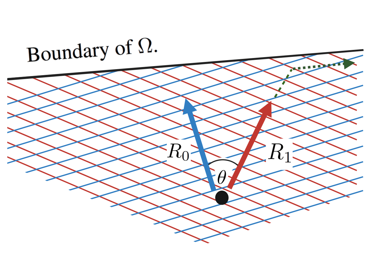
We can visualise it as follows:
Here the red arrow denotes the direction of R1 within Ω. Note that this direction corresponds to MR1, rather than R1, since Ω lies in a lower-dimensional affine subspace. Similarly, the red lines correspond to the level sets of R1, i.e. the directions we can move in without changing R1.
Now, if R1 is a proxy reward, then we may assume that there is also some (unknown) true reward function R0. This reward also induces a linear function on Ω, and the angle between them is θ:
Suppose we pick a random point ηπ in Ω, and then move in a direction that increases ηπ⋅R1. This corresponds to picking a random policy π, and then modifying it in a direction that increases JR1(π). In particular, let us consider what happens to the true reward function R0, as we move in the direction that most rapidly increases the proxy reward R1.
To start with, if we are in the interior of Ω (i.e., not close to any constraints), then the direction that most rapidly increases R1 is to move parallel to MR1. Moreover, if the angle θ between MR1 and MR0 is no more than π/2, then this is guaranteed to also increase the value of R0. To see this, consider the following diagram:
However, as we move parallel to MR1, we will eventually hit the boundary of Ω. When we do this, the direction that most rapidly increases R1 will no longer be parallel to MR1. Instead, it will be parallel to the projection of R1 onto the boundary of Ω that we just hit. Moreover, if we keep moving in this direction, then we might no longer be increasing the true reward R0. To see this, consider the following diagram:
The dashed green line corresponds to the path that most rapidly increases R1. As we move along this path, R0 initially increases. However, after the path hits the boundary of Ω and changes direction, R0 will instead start to decrease. Thus, if we were to plot JR1(π) and JR0(π) over time, we would get a plot that looks roughly like this:
Next, it is important to note that R0 is not guaranteed to decrease after we hit the boundary of Ω. To see this, consider the following diagram:
The dashed green line again corresponds to the path that most rapidly increases R1. As we move along this path, R0 will increase both before and after the path has hit the boundary of Ω. If we were to plot JR1(π) and JR0(π) over time, we would get a plot that looks roughly like this:
The next thing to note is that we will not just hit the boundary of Ω once. If we pick a random point ηπ in Ω, and keep moving in the direction that most rapidly increases ηπ⋅R1 until we have found the maximal value of R1 in Ω, then we will hit the boundary of Ω over and over again. Each time we hit this boundary we will change the direction that we are moving in, and each time this happens, there is a risk that we will start moving in a direction that decreases R0.
Goodharting corresponds to the case where we follow a path through Ω along which R0 initially increases, but eventually starts to decrease. As we have seen, this must be caused by the boundaries of Ω.
We may now ask; under what conditions do these boundaries force the path of steepest ascent (of R1) to move in a direction that decreases R0? By inspecting the above diagrams, we can see that this depends on the angle between the normal vector of that boundary and MR1, and the angle between MR1 and MR0. In particular, in order for R0 to start decreasing, it has to be the case that the angle between MR1 and MR0 is larger than the angle between MR1 and the normal vector of the boundary of Ω. This immediately tells us that if the angle between MR1 and MR0 is small, then Goodharting will be less likely to occur.
Moreover, as the angle between MR1 and the normal vector of the boundary of Ω becomes smaller, Goodharting should be correspondingly more likely to occur. In our paper, Proposition 3 tells us that this angle will decrease monotonically along the path of steepest ascent (of R1). As such, Goodharting will get more and more likely the further we move along the path of steepest ascent. This explains why Goodharting becomes more likely when more optimisation pressure is applied.
How can we use this intuition?
Preventing Goodharting is difficult because we only have access to the proxy reward. If we only observe R1, we don't know whether we are in the situation on the left or the situation on the right:
However, we might detect that there is a danger of Goodharting: if we have a bound on the angle θ between the true and the proxy, then we can detect when there is at least one policy within a cone of θ around R1 whose return goes down. This is the idea for the pessimistic early stopping algorithm we have developed. Specifically, we track the current direction of optimisation relative to the proxy reward R1 given by αi+2=arg(ηi+2−ηi+1,R1), in the occupancy measure space:
If α+θ>π/2, or equivalently, cos(α)<cos(π/2−θ)=sin(θ), there is a possibility of Goodharting - since pessimistically, we are moving opposite to some possible true reward R0.
In the interior of the polytope Ω, we know that the increase in return is given by the product of how much we moved and the magnitude of the (projected) reward vector: JR1(πi+1)−JR1(πi)=||ηi+1−ηi||⋅||MR1||. In general, it has to be rescaled by the current direction of optimisation: JR1(πi+2)−JR1(πi+1)=cos(αi+2)||ηi+2−ηi+1||⋅||MR1||.
Therefore, assuming that the LHS of the following inequality is non-increasing (Proposition 3 in the paper again):
JR1(πi+1)−JR1(πi)||ηπi+1−ηπi||<sin(θ)||MR1||we can simply stop first i that satisfies it. This is the optimal (last possible) point where we still provably avoid Goodharting.
What's next?
Early-stopping can, unfortunately, lose out on quite a lot of reward, so we think this particular method can be best used in situations where it is much more important to prevent Goodharting than to get good performance in absolute terms. It is also expensive to compute the occupancy measure η and the angle θ. Still, the algorithm can be improved in many directions: for example, we might be able to construct a training algorithm where we alternate between (1) training a model and (2) collecting more data about the reward function. In this way, we collect just enough information for training to proceed, without ever falling into Goodharting. We write about some of those possibilities in the paper but leave the details for future work.