This post covers work done by several researchers at, visitors to and collaborators of ARC, including Zihao Chen, George Robinson, David Matolcsi, Jacob Stavrianos, Jiawei Li and Michael Sklar. Thanks to Aryan Bhatt, Gabriel Wu, Jiawei Li, Lee Sharkey, Victor Lecomte and Zihao Chen for comments.
In the wake of recent debate about pragmatic versus ambitious visions for mechanistic interpretability, ARC is sharing some models we've been studying that, in spite of their tiny size, serve as challenging test cases for any ambitious interpretability vision. The models are RNNs and transformers trained to perform algorithmic tasks, and range in size from 8 to 1,408 parameters. The largest model that we believe we more-or-less fully understand has 32 parameters; the next largest model that we have put substantial effort into, but have failed to fully understand, has 432 parameters. The models are available here:
We think that the "ambitious" side of the mechanistic interpretability community has historically underinvested in "fully understanding slightly complex models" compared to "partially understanding incredibly complex models". There has been some prior work aimed at full understanding, for instance on models trained to perform paren balancing, modular addition and more general group operations, but we still don't think the field is close to being able to fully understand our models (at least, not in the sense we discuss in this post). If we are going to one day fully understand multi-billion-parameter LLMs, we probably first need to reach the point where fully understanding models with a few hundred parameters is pretty easy; we hope that AlgZoo will spur research to either help us reach that point, or help us reckon with the magnitude of the challenge we face.
One likely reason for this underinvestment is lingering philosophical confusion over the meaning of "explanation" and "full understanding". Our current perspective at ARC is that, given a model that has been optimized for a particular loss, an "explanation" of the model amounts to a mechanistic estimate of the model's loss. We evaluate mechanistic estimates in one of two ways. We use surprise accounting to determine whether we have achieved a full understanding; but for practical purposes, we simply look at mean squared error as a function of compute, which allows us to compare the estimate with sampling.
In the rest of this post, we will:
Review our perspective on mechanistic estimates as explanations, including our two ways of evaluating mechanistic estimates
Walk through three AlgZoo RNNs that we've studied, the smallest of which we fully understand, and the largest of which we don't
Conclude with some thoughts on how ARC's approach relates to ambitious mechanistic interpretability
Mechanistic estimates as explanations
Models from AlgZoo are trained to perform a simple algorithmic task, such as calculating the position of the second-largest number in a sequence. To explain why such a model has good performance, we can produce a mechanistic estimate of its accuracy.[1] By "mechanistic", we mean that the estimate reasons deductively based on the structure of the model, in contrast to a sampling-based estimate, which makes inductive inferences about the overall performance from individual examples.[2] Further explanation of this concept can be found here.
Not all mechanistic estimates are high quality. For example, if the model had to choose between 10 different numbers, before doing any analysis at all, we might estimate the accuracy of the model to be 10%. This would be a mechanistic estimate, but a very crude one. So we need some way to evaluate the quality of a mechanistic estimate. We generally do this using one of two methods:
Mean squared error versus compute. The more conceptually straightforward way to evaluate a mechanistic estimate is to simply ask how close it gets to the model's actual accuracy. The more compute-intensive the mechanistic estimate, the closer it should get to the actual accuracy. Our matching sampling principle is roughly the following conjecture: there is a mechanistic estimation procedure that (given suitable advice) performs at least as well as random sampling in mean squared error for any given computational budget.
Surprise accounting. This is an information-theoretic metric that asks: how surprising is the model's actual accuracy, now that we have access to the mechanistic estimate? We accrue surprise in one of two ways: either the estimate itself performed some kind of calculation or check with a surprising result, or the model's actual accuracy is still surprising even after accounting for the mechanistic estimate and its uncertainty. Further explanation of this idea can be found here.
Surprise accounting is useful because it gives us a notion of "full understanding": a mechanistic estimate with as few bits of total surprise as the number of bits of optimization used to select the model. On the other hand, mean squared error versus compute is more relevant to applications such as low probability estimation, as well as being easier to work with. We have been increasingly focused on matching the mean squared error of random sampling, which remains a challenging baseline, although we generally consider this to be easier than achieving a full understanding. The two metrics are often closely related, and we will walk through examples of both metrics in the case study below.
For most of the larger models from AlgZoo (including the 432-parameter model M16,10 discussed below), we would consider it a major research breakthrough if we were able to produce a mechanistic estimate that matched the performance of random sampling under the mean squared error versus compute metric.[3] It would be an even harder accomplishment to achieve a full understanding under the surprise accounting metric, but we are less focused on this.
Case study: 2nd argmax RNNs
The models in AlgZoo are divided into four families, based on the task they have been trained to perform. The family we have spent by far the longest studying is the family of models trained to find the position of the second-largest number in a sequence, which we call the "2nd argmax" of the sequence.
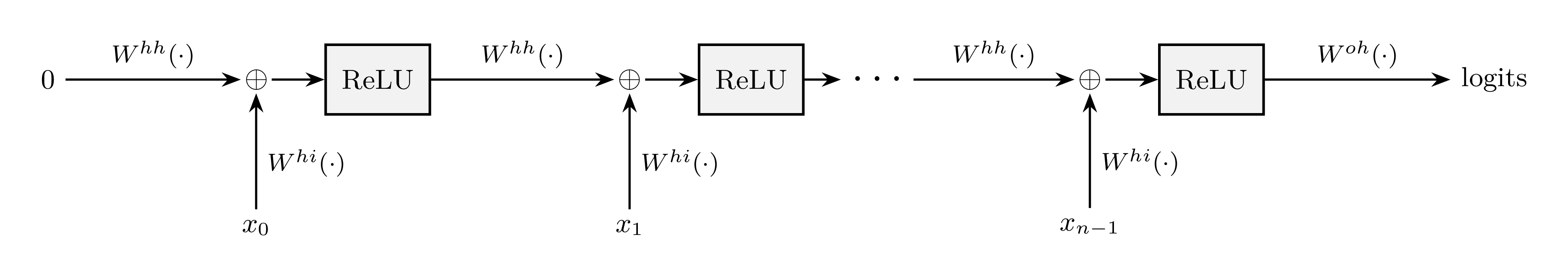
The models in this family are parameterized by a hidden size d and a sequence length n. The model Md,n is a 1-layer ReLU RNN with d hidden neurons that takes in a sequence of n real numbers and produces a vector of logit probabilities of length n. It has three parameter matrices:
the input-to-hidden matrix Whi∈Rd×1
the hidden-to-hidden matrix Whh∈Rd×d
the hidden-to-output matrix Woh∈Rn×d
The logits of Md,n on input sequence x0,…,xn−1∈R are computed as follows:
h0=0∈Rd
ht+1=ReLU(Whhht+Whixt) for t=0,…,n−1
logits=Wohhn
Diagrammatically:
Each model in this family is trained to make the largest logit be the one that corresponds to the position of second-largest input, using softmax cross-entropy loss.
The models we'll discuss here are M2,2, M4,3 and M16,10. For each of these models, we'd like to understand why the trained model has high accuracy on standard Gaussian input sequences.
Hidden size 2, sequence length 2
The model M2,2 can be loaded in AlgZoo using zoo_2nd_argmax(2, 2). It has 10 parameters and almost perfect 100% accuracy, with an error rate of roughly 1 in 13,000. This means that the difference between the model's logits, Δ(x0,x1):=logits(x0,x1)1−logits(x0,x1)0,is almost always negative when x1>x0 and positive when x0>x1. We'd like to mechanistically explain why the model has this property.
To do this, note first that because the model uses ReLU activations and there are no biases, Δ is a piecewise linear function of x0 and x1 in which the pieces are bounded by rays through the origin in the x0-x1 plane.
Now, we can "standardize" the model to obtain an exactly equivalent model for which the entries of Whi lie in {±1}, by rescaling the neurons of the hidden state. Once we do this, we see that Whi=(+1−1),Whh∈([−1,0)[1,∞)[1,∞)[−1,0))andWoh∈((0,∞)(−∞,0)(−∞,0)(0,∞)).
From these observations, we can prove that, on each linear piece of Δ, Δ(x0,x1)=a0x0−a1x1with a0,a1>0, and moreover, the pieces of Δ are arranged in the x0-x1 plane according to the following diagram:
Here, a double arrow indicates that a boundary lies somewhere between its neighboring axis and the dashed line x0=x1, but we don't need to worry about exactly where it lies within this range.
Looking at the coefficients of each linear piece, we observe that:
In the two blue regions, we have a0<a1
In the two green regions, we have a0>a1
In the two yellow regions, we have a0≈a1 to within around 1 part in 211
This implies that:
Δ(x0,x1)<0 in the blue and green regions above the line x0=x1
Δ(x0,x1)>0 in the blue and green regions below the line x0=x1
Δ(x0,x1) is approximately proportional to x0−x1 in the two yellow regions
Together, these imply that the model has almost 100% accuracy. More precisely, the error rate is the fraction of the unit disk lying between the model's decision boundary and the line x0=x1, which is around 1 in 2π×211≈13,000. This is very close to the model's empirically-measured error rate.
Mean squared error versus compute. Using only a handful of computational operations, we were able to mechanistically estimate the model's accuracy to within under 1 part in 13,000, which would have taken tens of thousands of samples. So our mechanistic estimate was much more computationally efficient than random sampling. Moreover, we could have easily produced a much more precise estimate (exact to within floating point error) by simply computing how close a0 and a1 were in the two yellow regions.
Surprise accounting. As explained here, the total surprise decomposes into the surprise of the explanation plus the surprise given the explanation. The surprise given the explanation is close to 0 bits, since the calculation was essentially exact. For the surprise of the explanation, we can walk through the steps we took:
We "standardized" the model, which simply replaced the model with an exactly equivalent one. This did not depend on the model's parameters at all, and so doesn't incur any surprise.
We checked the signs of all 10 of the model's parameters, and whether or not each of the 4 entries of Whh was greater than or less than 1 in magnitude, incurring 14 bits of surprise.
We deduced from this the form of the piecewise linear function Δ. This was another step that didn't depend on the model's parameters and so doesn't incur any surprise.
We checked which of the two linear coefficients was larger in magnitude in each of the 4 blue and green regions, incurring 4 bits of surprise.
We checked that the two linear coefficients were equal in magnitude in each of the 2 yellow regions to within 1 part in 211, incurring around 22 bits of surprise.
Adding this up, the total surprise is around 40 bits. This plausibly matches the number of bits of optimization used to select the model, since it was probably necessary to optimize the linear coefficients in the yellow regions to be almost equal. So we can be relatively comfortable in saying that we have achieved a full understanding.
Note that our analysis here was pretty "brute force": we essentially checked each linear region of Δ one by one, with a little work up front to reduce the total number of checks required. Even though we consider this to constitute a full understanding in this case, we would not draw the same conclusion for much deeper models. This is because the number of regions would grow exponentially with depth, making the number of bits of surprise far larger than the number of bits taken up by the weights of the model (which is an upper bound on the number of bits of optimization used to select the model). The same exponential blowup would also prevent us from matching the efficiency of sampling at reasonable computational budgets.
Finally, it is interesting to note that our analysis allows us to construct a model by hand that gets exactly 100% accuracy, by taking Whi=(+1−1),Whh=(−1+1+1−1)andWoh=(+1−1−1+1).
Hidden size 4, sequence length 3
The model M4,3 can be loaded in AlgZoo using zoo_2nd_argmax(4, 3). It has 32 parameters and an accuracy of 98.5%.
Our analysis of M4,3 is broadly similar to our analysis of M2,2, but the model is already deep enough that we wouldn't consider a fully brute force explanation to be adequate. To deal with this, we exploit various approximate symmetries in the model to reduce the total number of computational operations as well as the surprise of the explanation. Our full analysis can be found in these sets of notes:
In the second set of notes, we provide two different mechanistic estimates for the model's accuracy that use different amounts of compute, depending on which approximate symmetries are exploited. We analyze both estimates according to our two metrics. We find that we are able to roughly match the computational efficiency of sampling,[4] and we think we more-or-less have a full understanding, although this is less clear.
Finally, our analysis once again allows us to construct an improved model by hand, which has 99.99% accuracy.[5]
Hidden size 16, sequence length 10
The model M16,10 can be loaded in AlgZoo using example_2nd_argmax().[6] It has 432 parameters and an accuracy of 95.3%.
This model is deep enough that a brute force approach is no longer viable. Instead, we look for "features" in the activation space of the model's hidden state.
After rescaling the neurons of the hidden state, we notice an approximately isolated subcircuit formed by neurons 2 and 4, with no strong connections to the outputs of any other neurons: Whi(2,4)≈(0+1),Whh(2,4),(2,4)≈(+1+1−1−1)andWhh(2,4),(0,1,3,…)≈(0…0…).
It follows that after unrolling the RNN for t steps:
Neuron 2 is approximately max(0,x0,…,xt−2)
Neuron 4 is approximately max(0,x0,…,xt−1)−max(0,x0,…,xt−2)
This can be proved by induction using the identity ReLU(a−b)=max(a,b)−b for neuron 4.
Next, we notice that neurons 6 and 7 fit into a larger approximately isolated subcircuit together with neurons 2 and 4: Whi(6,7)≈(−1−1),Whh(6,7),(2,4)≈(+10+1+1)andWhh(6,7),(0,1,3,…)≈(0…0…).
Using the same identity, it follows that after unrolling the RNN for t steps:
Neuron 6 is approximately max(0,x0,…,xt−3,xt−1)−xt−1
Neuron 7 is approximately max(0,x0,…,xt−1)−xt−1
We can keep going, and add in neuron 1 to the subcircuit: Whi(1)≈(−1),Whh(1),(2,4,6,7)≈(+1+1+1−1)andWhh(1),(0,1,3,…)≈(0…).
Hence after unrolling the RNN for t steps, neuron 1 is approximately max(0,x0,…,xt−4,xt−2,xt−1)−xt−1,forming another "leave-one-out-maximum" feature (minus the most recent input).
In fact, by generalizing this idea, we can construct a model by hand that uses 22 hidden neurons to form all 10 leave-one-out-maximum features, and leverages these to achieve an accuracy of 99%.[7]
Unfortunately, however, it is challenging to go much further than this:
We have exploited the approximate weight sparsity of 5 of the hidden neurons, but most of the remaining 11 hidden neurons are more densely connected.
We have produced a handcrafted model with high accuracy, but we have not produced a correspondence between most of hidden neurons of the trained model and the hidden neurons of the handcrafted model.
We have used approximations in our analysis, but have not dealt with the approximation error, which gets increasingly significant as we consider more complex neurons.
Fundamentally, even though we have some understanding of the model, our explanation is incomplete because we not have not turned this understanding into an adequate mechanistic estimate of the model's accuracy.
Ultimately, to produce a mechanistic estimate for the accuracy of this model that is competitive with sampling (or that constitutes a full understanding), we expect we would have to somehow combine this kind of feature analysis with elements of the "brute force after exploiting symmetries" approach used for the models M2,2 and M4,3, and to do so in a primarily algorithmic way. This is why we consider producing such a mechanistic estimate to be a formidable research challenge.
Some notes with further discussion of this model can be found here:
The models in AlgZoo are small, but for all but the tiniest of them, it is a considerable challenge to mechanistically estimate their accuracy competitively with sampling, let alone fully understand them in the sense of surprise accounting. At the same time, AlgZoo models are trained on tasks that can easily be performed by LLMs, so fully understanding them is practically a prerequisite for ambitious LLM interpretability. Overall, we would be keen to see other ambitious-oriented researchers explore our models, and more concretely, we would be excited to see better mechanistic estimates for our models in the sense of mean squared error versus compute. One specific challenge we pose is the following.
Challenge: Design a method for mechanistically estimating the accuracy of the 432-parameter model M16,10[8] that matches the performance of random sampling in terms of mean squared error versus compute. A cheap way to measure mean squared error is to add noise to the model's weights (enough to significantly alter the model's accuracy) and check the squared error of the method on average over the choice of noisy model.[9]
How does ARC's broader approach relate to this? The analysis we have presented here is relatively traditional mechanistic interpretability, but we think of this analysis mainly as a warm-up. Ultimately, we seek a scalable, algorithmic approach to producing mechanistic estimates, which we have been pursuing in our recent work. Furthermore, we are ambitious in the sense that we would like to fully exploit the structure present in models to mechanistically estimate any quantity of interest.[10] Thus our approach is best described as "ambitious" and "mechanistic", but perhaps not as "interpretability".
Technically, the model was trained to minimize cross-entropy loss (with a small amount of weight decay), not to maximize accuracy, but the two are closely related, so we will gloss over this distinction. ↩︎
The term "mechanistic estimate" is essentially synonymous with "heuristic explanation" as used here or "heuristic argument" as used here, except that it refers more naturally to a numeric output rather than the process used to produce it, and has other connotations we now prefer. ↩︎
An estimate for a single model could be close by chance, so the method should match sampling on average over random seeds. ↩︎
To assess the mean squared error of our method, we add noise to the model's weights and check the squared error of our method on average over the choice of noisy model. ↩︎
This handcrafted model can be loaded in AlgZoo using handcrafted_2nd_argmax(3). Credit to Michael Sklar for correspondence that led to this construction. ↩︎
We treat this model as separate from the "official" model zoo because it was trained before we standardized our codebase. Credit to Zihao Chen for originally training and analyzing this model. The model from the zoo that can be loaded using zoo_2nd_argmax(16, 10) has the same architecture, and is probably fairly similar, but we have not analyzed it. ↩︎
This handcrafted model can be loaded in AlgZoo using handcrafted_2nd_argmax(10). Note that this handcrafted model has more hidden neurons than the trained model M16,10. ↩︎
The specific model we are referring to can be be loaded in AlgZoo using example_2nd_argmax(). Additional 2nd argmax models with the same architecture, which a good method should also work well on, can be loaded using zoo_2nd_argmax(16, 10, seed=seed) for seed equal to 0, 1, 2, 3 or 4. ↩︎
A better but more expensive way to measure mean squared error is to instead average over random seeds used to train the model. ↩︎
We are ambitious in this sense because of our worst-case theoretical methodology, but at the same time, we are focused more on applications such as low probability estimation than on understanding inherently, for which partial success could result in pragmatic wins. ↩︎
This post covers work done by several researchers at, visitors to and collaborators of ARC, including Zihao Chen, George Robinson, David Matolcsi, Jacob Stavrianos, Jiawei Li and Michael Sklar. Thanks to Aryan Bhatt, Gabriel Wu, Jiawei Li, Lee Sharkey, Victor Lecomte and Zihao Chen for comments.
In the wake of recent debate about pragmatic versus ambitious visions for mechanistic interpretability, ARC is sharing some models we've been studying that, in spite of their tiny size, serve as challenging test cases for any ambitious interpretability vision. The models are RNNs and transformers trained to perform algorithmic tasks, and range in size from 8 to 1,408 parameters. The largest model that we believe we more-or-less fully understand has 32 parameters; the next largest model that we have put substantial effort into, but have failed to fully understand, has 432 parameters. The models are available here:
[ AlgZoo GitHub repo ]
We think that the "ambitious" side of the mechanistic interpretability community has historically underinvested in "fully understanding slightly complex models" compared to "partially understanding incredibly complex models". There has been some prior work aimed at full understanding, for instance on models trained to perform paren balancing, modular addition and more general group operations, but we still don't think the field is close to being able to fully understand our models (at least, not in the sense we discuss in this post). If we are going to one day fully understand multi-billion-parameter LLMs, we probably first need to reach the point where fully understanding models with a few hundred parameters is pretty easy; we hope that AlgZoo will spur research to either help us reach that point, or help us reckon with the magnitude of the challenge we face.
One likely reason for this underinvestment is lingering philosophical confusion over the meaning of "explanation" and "full understanding". Our current perspective at ARC is that, given a model that has been optimized for a particular loss, an "explanation" of the model amounts to a mechanistic estimate of the model's loss. We evaluate mechanistic estimates in one of two ways. We use surprise accounting to determine whether we have achieved a full understanding; but for practical purposes, we simply look at mean squared error as a function of compute, which allows us to compare the estimate with sampling.
In the rest of this post, we will:
Mechanistic estimates as explanations
Models from AlgZoo are trained to perform a simple algorithmic task, such as calculating the position of the second-largest number in a sequence. To explain why such a model has good performance, we can produce a mechanistic estimate of its accuracy.[1] By "mechanistic", we mean that the estimate reasons deductively based on the structure of the model, in contrast to a sampling-based estimate, which makes inductive inferences about the overall performance from individual examples.[2] Further explanation of this concept can be found here.
Not all mechanistic estimates are high quality. For example, if the model had to choose between 10 different numbers, before doing any analysis at all, we might estimate the accuracy of the model to be 10%. This would be a mechanistic estimate, but a very crude one. So we need some way to evaluate the quality of a mechanistic estimate. We generally do this using one of two methods:
Surprise accounting is useful because it gives us a notion of "full understanding": a mechanistic estimate with as few bits of total surprise as the number of bits of optimization used to select the model. On the other hand, mean squared error versus compute is more relevant to applications such as low probability estimation, as well as being easier to work with. We have been increasingly focused on matching the mean squared error of random sampling, which remains a challenging baseline, although we generally consider this to be easier than achieving a full understanding. The two metrics are often closely related, and we will walk through examples of both metrics in the case study below.
For most of the larger models from AlgZoo (including the 432-parameter model M16,10 discussed below), we would consider it a major research breakthrough if we were able to produce a mechanistic estimate that matched the performance of random sampling under the mean squared error versus compute metric.[3] It would be an even harder accomplishment to achieve a full understanding under the surprise accounting metric, but we are less focused on this.
Case study: 2nd argmax RNNs
The models in AlgZoo are divided into four families, based on the task they have been trained to perform. The family we have spent by far the longest studying is the family of models trained to find the position of the second-largest number in a sequence, which we call the "2nd argmax" of the sequence.
The models in this family are parameterized by a hidden size d and a sequence length n. The model Md,n is a 1-layer ReLU RNN with d hidden neurons that takes in a sequence of n real numbers and produces a vector of logit probabilities of length n. It has three parameter matrices:
The logits of Md,n on input sequence x0,…,xn−1∈R are computed as follows:
Diagrammatically:
Each model in this family is trained to make the largest logit be the one that corresponds to the position of second-largest input, using softmax cross-entropy loss.
The models we'll discuss here are M2,2, M4,3 and M16,10. For each of these models, we'd like to understand why the trained model has high accuracy on standard Gaussian input sequences.
Hidden size 2, sequence length 2
The model M2,2 can be loaded in AlgZoo using
zoo_2nd_argmax(2, 2). It has 10 parameters and almost perfect 100% accuracy, with an error rate of roughly 1 in 13,000. This means that the difference between the model's logits,Δ(x0,x1):=logits(x0,x1)1−logits(x0,x1)0,is almost always negative when x1>x0 and positive when x0>x1. We'd like to mechanistically explain why the model has this property.
To do this, note first that because the model uses ReLU activations and there are no biases, Δ is a piecewise linear function of x0 and x1 in which the pieces are bounded by rays through the origin in the x0-x1 plane.
Now, we can "standardize" the model to obtain an exactly equivalent model for which the entries of Whi lie in {±1}, by rescaling the neurons of the hidden state. Once we do this, we see that
Whi=(+1−1),Whh∈([−1,0)[1,∞)[1,∞)[−1,0))andWoh∈((0,∞)(−∞,0)(−∞,0)(0,∞)).
From these observations, we can prove that, on each linear piece of Δ,
Δ(x0,x1)=a0x0−a1x1with a0,a1>0, and moreover, the pieces of Δ are arranged in the x0-x1 plane according to the following diagram:
Here, a double arrow indicates that a boundary lies somewhere between its neighboring axis and the dashed line x0=x1, but we don't need to worry about exactly where it lies within this range.
Looking at the coefficients of each linear piece, we observe that:
This implies that:
Together, these imply that the model has almost 100% accuracy. More precisely, the error rate is the fraction of the unit disk lying between the model's decision boundary and the line x0=x1, which is around 1 in 2π×211≈13,000. This is very close to the model's empirically-measured error rate.
Mean squared error versus compute. Using only a handful of computational operations, we were able to mechanistically estimate the model's accuracy to within under 1 part in 13,000, which would have taken tens of thousands of samples. So our mechanistic estimate was much more computationally efficient than random sampling. Moreover, we could have easily produced a much more precise estimate (exact to within floating point error) by simply computing how close a0 and a1 were in the two yellow regions.
Surprise accounting. As explained here, the total surprise decomposes into the surprise of the explanation plus the surprise given the explanation. The surprise given the explanation is close to 0 bits, since the calculation was essentially exact. For the surprise of the explanation, we can walk through the steps we took:
Adding this up, the total surprise is around 40 bits. This plausibly matches the number of bits of optimization used to select the model, since it was probably necessary to optimize the linear coefficients in the yellow regions to be almost equal. So we can be relatively comfortable in saying that we have achieved a full understanding.
Note that our analysis here was pretty "brute force": we essentially checked each linear region of Δ one by one, with a little work up front to reduce the total number of checks required. Even though we consider this to constitute a full understanding in this case, we would not draw the same conclusion for much deeper models. This is because the number of regions would grow exponentially with depth, making the number of bits of surprise far larger than the number of bits taken up by the weights of the model (which is an upper bound on the number of bits of optimization used to select the model). The same exponential blowup would also prevent us from matching the efficiency of sampling at reasonable computational budgets.
Finally, it is interesting to note that our analysis allows us to construct a model by hand that gets exactly 100% accuracy, by taking
Whi=(+1−1),Whh=(−1+1+1−1)andWoh=(+1−1−1+1).
Hidden size 4, sequence length 3
The model M4,3 can be loaded in AlgZoo using
zoo_2nd_argmax(4, 3). It has 32 parameters and an accuracy of 98.5%.Our analysis of M4,3 is broadly similar to our analysis of M2,2, but the model is already deep enough that we wouldn't consider a fully brute force explanation to be adequate. To deal with this, we exploit various approximate symmetries in the model to reduce the total number of computational operations as well as the surprise of the explanation. Our full analysis can be found in these sets of notes:
In the second set of notes, we provide two different mechanistic estimates for the model's accuracy that use different amounts of compute, depending on which approximate symmetries are exploited. We analyze both estimates according to our two metrics. We find that we are able to roughly match the computational efficiency of sampling,[4] and we think we more-or-less have a full understanding, although this is less clear.
Finally, our analysis once again allows us to construct an improved model by hand, which has 99.99% accuracy.[5]
Hidden size 16, sequence length 10
The model M16,10 can be loaded in AlgZoo using
example_2nd_argmax().[6] It has 432 parameters and an accuracy of 95.3%.This model is deep enough that a brute force approach is no longer viable. Instead, we look for "features" in the activation space of the model's hidden state.
After rescaling the neurons of the hidden state, we notice an approximately isolated subcircuit formed by neurons 2 and 4, with no strong connections to the outputs of any other neurons:
Whi(2,4)≈(0+1),Whh(2,4),(2,4)≈(+1+1−1−1)andWhh(2,4),(0,1,3,…)≈(0…0…).
It follows that after unrolling the RNN for t steps:
This can be proved by induction using the identity ReLU(a−b)=max(a,b)−b for neuron 4.
Next, we notice that neurons 6 and 7 fit into a larger approximately isolated subcircuit together with neurons 2 and 4:
Whi(6,7)≈(−1−1),Whh(6,7),(2,4)≈(+10+1+1)andWhh(6,7),(0,1,3,…)≈(0…0…).
Using the same identity, it follows that after unrolling the RNN for t steps:
We can keep going, and add in neuron 1 to the subcircuit:
Whi(1)≈(−1),Whh(1),(2,4,6,7)≈(+1+1+1−1)andWhh(1),(0,1,3,…)≈(0…).
Hence after unrolling the RNN for t steps, neuron 1 is approximately
max(0,x0,…,xt−4,xt−2,xt−1)−xt−1,forming another "leave-one-out-maximum" feature (minus the most recent input).
In fact, by generalizing this idea, we can construct a model by hand that uses 22 hidden neurons to form all 10 leave-one-out-maximum features, and leverages these to achieve an accuracy of 99%.[7]
Unfortunately, however, it is challenging to go much further than this:
Fundamentally, even though we have some understanding of the model, our explanation is incomplete because we not have not turned this understanding into an adequate mechanistic estimate of the model's accuracy.
Ultimately, to produce a mechanistic estimate for the accuracy of this model that is competitive with sampling (or that constitutes a full understanding), we expect we would have to somehow combine this kind of feature analysis with elements of the "brute force after exploiting symmetries" approach used for the models M2,2 and M4,3, and to do so in a primarily algorithmic way. This is why we consider producing such a mechanistic estimate to be a formidable research challenge.
Some notes with further discussion of this model can be found here:
Conclusion
The models in AlgZoo are small, but for all but the tiniest of them, it is a considerable challenge to mechanistically estimate their accuracy competitively with sampling, let alone fully understand them in the sense of surprise accounting. At the same time, AlgZoo models are trained on tasks that can easily be performed by LLMs, so fully understanding them is practically a prerequisite for ambitious LLM interpretability. Overall, we would be keen to see other ambitious-oriented researchers explore our models, and more concretely, we would be excited to see better mechanistic estimates for our models in the sense of mean squared error versus compute. One specific challenge we pose is the following.
Challenge: Design a method for mechanistically estimating the accuracy of the 432-parameter model M16,10[8] that matches the performance of random sampling in terms of mean squared error versus compute. A cheap way to measure mean squared error is to add noise to the model's weights (enough to significantly alter the model's accuracy) and check the squared error of the method on average over the choice of noisy model.[9]
How does ARC's broader approach relate to this? The analysis we have presented here is relatively traditional mechanistic interpretability, but we think of this analysis mainly as a warm-up. Ultimately, we seek a scalable, algorithmic approach to producing mechanistic estimates, which we have been pursuing in our recent work. Furthermore, we are ambitious in the sense that we would like to fully exploit the structure present in models to mechanistically estimate any quantity of interest.[10] Thus our approach is best described as "ambitious" and "mechanistic", but perhaps not as "interpretability".
Technically, the model was trained to minimize cross-entropy loss (with a small amount of weight decay), not to maximize accuracy, but the two are closely related, so we will gloss over this distinction. ↩︎
The term "mechanistic estimate" is essentially synonymous with "heuristic explanation" as used here or "heuristic argument" as used here, except that it refers more naturally to a numeric output rather than the process used to produce it, and has other connotations we now prefer. ↩︎
An estimate for a single model could be close by chance, so the method should match sampling on average over random seeds. ↩︎
To assess the mean squared error of our method, we add noise to the model's weights and check the squared error of our method on average over the choice of noisy model. ↩︎
This handcrafted model can be loaded in AlgZoo using
handcrafted_2nd_argmax(3). Credit to Michael Sklar for correspondence that led to this construction. ↩︎We treat this model as separate from the "official" model zoo because it was trained before we standardized our codebase. Credit to Zihao Chen for originally training and analyzing this model. The model from the zoo that can be loaded using
zoo_2nd_argmax(16, 10)has the same architecture, and is probably fairly similar, but we have not analyzed it. ↩︎This handcrafted model can be loaded in AlgZoo using
handcrafted_2nd_argmax(10). Note that this handcrafted model has more hidden neurons than the trained model M16,10. ↩︎The specific model we are referring to can be be loaded in AlgZoo using
example_2nd_argmax(). Additional 2nd argmax models with the same architecture, which a good method should also work well on, can be loaded usingzoo_2nd_argmax(16, 10, seed=seed)forseedequal to 0, 1, 2, 3 or 4. ↩︎A better but more expensive way to measure mean squared error is to instead average over random seeds used to train the model. ↩︎
We are ambitious in this sense because of our worst-case theoretical methodology, but at the same time, we are focused more on applications such as low probability estimation than on understanding inherently, for which partial success could result in pragmatic wins. ↩︎