My speculation for Omni-Grok in particular is that in settings like MNIST you already have two of the ingredients for grokking (that there are both memorising and generalising solutions, and that the generalising solution is more efficient), and then having large parameter norms at initialisation provides the third ingredient (generalising solutions are learned more slowly), for some reason I still don't know.

Higher weight norm means lower effective learning rate with Adam, no? In that paper they used a constant learning rate across weight norms, but Adam tries to normalize the gradients to be of size 1 per paramter, regardless of the size of the weights. So the weights change more slowly with larger initializations (especially since they constrain the weights to be of fixed norm by projecting after the Adam step). 

I mean, yeah, as your footnote says:

Another simpler but less illuminating way to put this is that higher serial reasoning depth can't be parallelized.^[1]

Transformers do get more computation per token on longer sequences, but they also don't get more serial depth, so I'm not sure if this is actually an issue in practice?

1. ^{^}

   [C]ompactly represent $f\circ g$ (f composed with g) in a way that makes computing $f\left(g\right(x\left)\right)$ more efficient for general choices of $f$ and $g$.

   As an aside, I actually can't think of any class of interesting functions with this property -- when reading the paper, the closest I could think of are functions on discrete sets (lol), polynomials (but simplifying these are often more expensive than just computing the terms serially), and rational functions (ditto)

    

I finally got around to reading the Mamba paper. H/t Ryan Greenblatt and Vivek Hebbar for helpful comments that got me unstuck. 

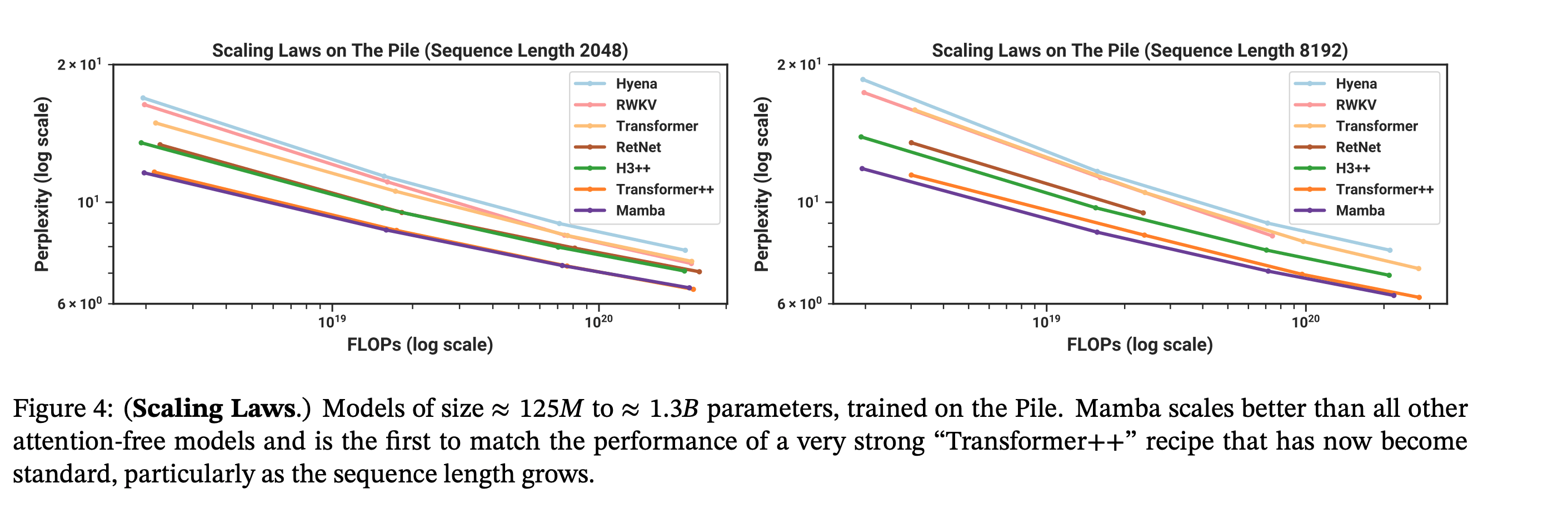
TL;DR: authors propose a new deep learning architecture for sequence modeling with scaling laws that match transformers while being much more efficient to sample from.

A brief historical digression

As of ~2017, the three primary ways people had for doing sequence modeling were RNNs, Conv Nets, and Transformers, each with a unique “trick” for handling sequence data: recurrence, 1d convolutions, and self-attention.
 

• RNNs are easy to sample from — to compute the logit for x_t+1, you only need the most recent hidden state h_t and the last token x_t, which means it’s both fast and memory efficient. RNNs generate a sequence of length L with O(1) memory and O(L) time. However, they’re super hard to train, because  you need to sequentially generate all the hidden states and then (reverse) sequentially calculate the gradients. The way you actually did this is called backpropogation through time — you basically unroll the RNN over time — which requires constructing a graph of depth equal to the sequence length. Not only was this slow, but the graph being so deep caused vanishing/exploding gradients without careful normalization. The strategy that people used was to train on short sequences and finetune on longer ones. That being said, in practice, this meant you couldn’t train on long sequences (>a few hundred tokens) at all. The best LSTMs for modeling raw audio could only handle being trained on ~5s of speech, if you chunk up the data into 25ms segments.
• Conv Nets had a fixed receptive field size and pattern, so weren’t that suited for long sequence  modeling. Also, generating each token takes O(L) time, assuming the receptive field is about the same size as the sequence. But they had significantly more stability (the depth was small, and could be as low as O(log(L))), which meant you could train them a lot easier. (Also, you could use FFT to efficiently compute the conv, meaning it trains one sequence in O(L log(L)) time.) That being said, you still couldn’t make them that big. The most impressive example was DeepMind’s WaveNet, conv net used to model human speech, and could handle up sequences up to 4800 samples … which was 0.3s of actual speech at 16k samples/second (note that most audio is sampled at 44k samples/second…), and even to to get to that amount, they had to really gimp the model’s ability to focus on particular inputs.
• Transformers are easy to train, can handle variable length sequences, and also allow the model to “decide” which tokens it should pay attention to. In addition to both being parallelizable and having relatively shallow computation graphs (like conv nets), you could do the RNN trick of pretraining on short sequences and then finetune on longer sequences to save even more compute. Transformers could be trained with comparable sequence length to conv nets but get much better performance; for example, OpenAI’s musenet was trained on sequence length 4096 sequences of MIDI files. But as we all know, transformers have the unfortunate downside of being expensive to sample from — it takes O(L) time and O(L) memory to generate a single token (!).

The better performance of transformers over conv nets and their ability to handle variable length data let them win out.

That being said, people have been trying to get around the O(L) time and memory requirements for transformers since basically their inception. For a while, people were super into sparse or linear attention of various kinds, which could reduce the per-token compute/memory requirements to O(log(L)) or O(1).

The what and why of Mamba

If the input -> hidden and hidden -> hidden map for RNNs were linear (h_t+1 = A h_t + B x_t), then it’d be possible to train an entire sequence in parallel — this is because you can just … compose the transformation with itself (computing A^k for k in 2…L-1) a bunch, and effectively unroll the graph with the convolutional kernel defined by A B, A^2 B, A^3 B, … A^{L-1} B. Not only can you FFT during training to get the O(L log (L)) time of a conv net forward/backward pass (as opposed to O(L^2) for the transformer), you still keep the O(1) sampling time/memory of the RNN!

The problem is that linear hidden state dynamics are kinda boring. For example, you can’t even learn to update your existing hidden state in a different way if you see particular tokens! And indeed, previous results gave scaling laws that were much worse than transformers in terms of performance/training compute. 

In Mamba, you basically learn a time varying A and B. The parameterization is a bit wonky here, because of historical reasons, but it goes something like: A_t is exp(-\delta(x_t) * exp(A)), B_t = \delta(x_t) B x_t, where \delta(x_t) = softplus ( W_\delta x_t). Also note that in Mamba, they also constrain A to be diagonal and W_\delta to be low rank, for computational reasons  

Since exp(A) is diagonal and has only positive entries, we can interpret the model as follows: \delta controls how much to “learn” from the current example — with high \delta, A_t approaches 0 and B_t is large, causing h_t+1 ~= B_t x_t, while with \delta approaching 0, A_t approaches 1 and B_t approaches 0, meaning h_t+1 ~= h_t.

Now, you can’t exactly unroll the hidden state as a convolution with a predefined convolution kernel anymore, but you can still efficiently compute the implied “convolution” using parallel scanning.

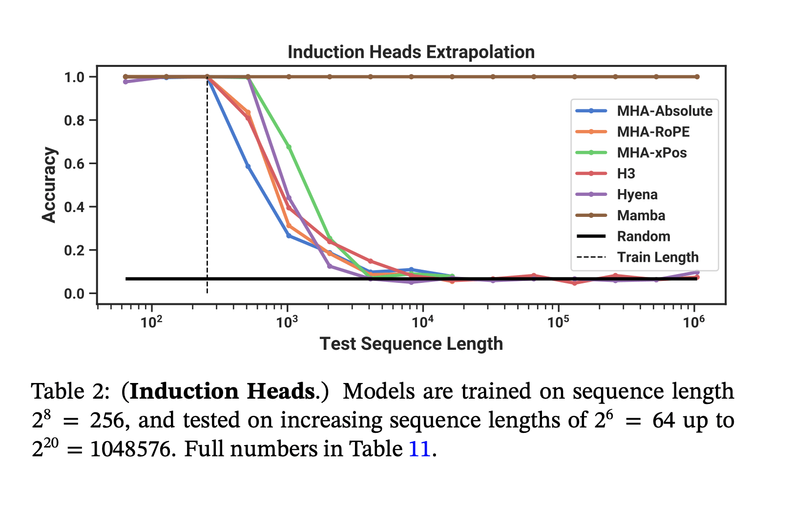
Despite being much cheaper to sample from, Mamba matches the pretraining flops efficiency of modern transformers (Transformer++ = the current SOTA open source Transformer with RMSNorm, a better learning rate schedule, and corrected AdamW hyperparameters, etc.). And on a toy induction task, it generalizes to much longer sequences than it was trained on.

So, about those capability externalities from mech interp...

Yes, those are the same induction heads from the Anthropic ICL paper! 

Like the previous Hippo and Hyena papers they cite mech interp as one of their inspirations, in that it inspired them to think about what the linear hidden state model could not model and how to fix that. I still don’t think mech interp has that much Shapley here (the idea of studying how models perform toy tasks is not new, and the authors don't even use induction metric or RRT task from the Olsson et al paper), but I'm not super sure on this.

IMO, this is line of work is the strongest argument for mech interp (or maybe interp in general) having concrete capabilities externalities. In addition, I think the previous argument Neel and I gave of "these advances are extremely unlikely to improve frontier models" feels substantially weaker now.

Is this a big deal?

I don't know, tbh.

Right, the step I missed on was that P(X|Y) = P(X|Z) for all y, z implies P(X|Z) = P(X). Thanks!

Hm, it sounds like you're claiming that if each pair of x, y, z are pairwise independent conditioned on the third variable, and p(x, y, z) =/= 0 for all x, y, z with nonzero p(x), p(y), p(z), then ?

I tried for a bit to show this but couldn't prove it, let alone the general case without strong invariance. My guess is I'm probably missing something really obvious. 

Probabilities of zero are extremely load-bearing for natural latents in the exact case, and probabilities near zero are load-bearing in the approximate case; if the distribution is zero nowhere, then it can only have a natural latent if the $X_i$’s are all independent (in which case the trivial variable is a natural latent).

I'm a bit confused why this is the case. It seems like in the theorems, the only thing "near zero" is that D_KL (joint, factorized) < epsilon ~= 0 . But you. can satisfy this quite easily even with all probabilities > 0. 

E.g. the trivial case where all variables are completely independents satisfies all the conditions of your theorem, but can clearly have every pair of probabilities > 0. Even in nontrivial cases, this is pretty easy (e.g. by mixing in irreducible noise with every variable).

After having spent a few hours playing with Opus, I think "slightly better than best public gpt-4" seems qualitatively correct -- both models tend to get tripped up on the same kinds of tasks, but Opus can inconsistently solve some tasks in my workflow that gpt-4 cannot. 

And yeah, it seems likely that I will also swap to Claude over ChatGPT. 

Thanks for doing this!

Fascinating, thanks for the update!

(I haven't had the chance to read part 3 in detail, and I also haven't checked the proofs except insofar as they seem reasonable on first viewing. Will probably have a lot more thoughts after I've had more time to digest.)

This is very cool work! I like the choice of U-AND task, which seems way more amenable to theoretical study (and is also a much more interesting task) than the absolute value task studied in Anthropic's Toy Model of Superposition (hereafter TMS). It's also nice to study this toy task with asymptotic theoretical analysis as opposed to the standard empirical analysis, thereby allowing you to use a different set of tools than usual. 

The most interesting part of the results was the discussion on the universality of universal calculation -- it reminds me of the interpretations of the lottery ticket hypothesis that claim some parts of the network happen to be randomly initialized to have useful features at the start. 

Some examples that are likely to be boolean-interpretable are bigram-finding circuits and induction heads. However, it's possible that most computations are continuous rather than boolean^[31].

My guess is that most computations are indeed closer to continuous than to boolean. While it's possible to construct boolean interpretations of bigram circuits or induction heads, my impression (having not looked at either in detail on real models) is that neither of these cleanly occur inside LMs. For example, induction heads demonstrate a wide variety of other behavior, and even on induction-like tasks, often seem to be implementing induction heuristics that involve some degree of semantic content. 

Consequently, I'd be especially interested in exploring either the universality of universal calculation, or the extension to arithmetic circuits (or other continuous/more continuous models of computation in superposition).

Some nitpicks:

The post would probably be a lot more readable if it were chunked into 4.  The 88 minute read time is pretty scary, and I'd like to comment only on the parts I've read. 

Section 2:

Two reasons why this loss function might be principled are

1. If there is reason to think of the model as a Gaussian probability model
2. If we would like our loss function to be basis independent

A big reason to use MSE as opposed to eps-accuracy in the Anthropic model is for optimization purposes (you can't gradient descent cleanly through eps-accuracy). 

Section 5:

4 How relevant are our results to real models?

This should be labeled as section 5. 

Appendix to the Appendix:

Here, $f_i$ always denotes the vector.

[..]

with \[\sigma_1\leq n\) with

(TeX compilation failure)