Thanks for doing this!
Since PaLM was basically a continuation of the scaling strategy derived from the Kaplan paper, it's not surprising that it basically continues the trend. (right?)
I'd be very interested to see how Chinchilla compares, since it claims to be using a superior scaling strategy.
That's my read. It continues the Kaplan scaling. The Kaplan scaling isn't wrong (everything really does scale that way if you train that way), it's just suboptimal. PaLM is not a surprise, neither in the compute cost nor in having capability-spikes (at least, if you've been paying attention and not handwaving them away).
The surprise here is perhaps showing how bad GB/DM communications are, that DM may have let GB piss away millions of dollars of TPU time. As one Googler put it, 'we find out about this stuff the same way you do - from Twitter'.
The difference between Chinchilla and Gopher was small but noticeable. Since the Kaplan and DM optimal scaling trajectories are like two lines with different slopes, should we perhaps expect the difference to get larger at greater scales?
So then... If before we looked at the Kaplan scaling and thought e.g. 50% chance that +6 OOMs would be enough... now we correct for the updated scaling laws and think 50% chance that, what, +4 OOMs would be enough? How big do you think the adjustment would be? (Maybe I can work it out by looking at some of those IsoX graphs in the paper?)
Depends on how you were getting to that +N OOMs number.
If you were looking at my post, or otherwise using the scaling laws to extrapolate how fast AI was improving on benchmarks (or subjective impressiveness), then the chinchilla laws means you should get there sooner. I haven't run the numbers on how much sooner.
If you were looking at Ajeya's neural network anchor (i.e. the one using the Kaplan scaling-laws, not the human-lifetime or evolution anchors), then you should now expect that AGI comes later. That model anchors the number of parameters in AGI to the number of synapses in the human brain, and then calculates how much compute you'd need to train a model of that size, if you were on the compute-optimal trajectory. With the chinchilla scaling laws, you need more data to train a compute-optimal model with a given number of parameters (data is proportional to parameters instead of parameters^0.7). So now it seems like it's going to be more expensive to train a compute-optimal model with 10^15 parameters, or however many parameteres AGI would need.
Ok so I tried running the numbers for the neural net anchor in my bio-anchors guesstimate replica.
Previously the neural network anchor used an exponent (alpha) of normal(0.8, 0.2) (first number is mean, second is standard deviation). I tried changing that to normal(1, 0.1) (smaller uncertainty because 1 is a more natural number, and some other evidence was already pointing towards 1). Also, the model previously said that a 1-trillion parameter model should be trained with 10^normal(11.2, 1.5) data points. I changed that to have a median at 21.2e12 parameters, since that's what the chinchilla paper recommends for a 1-trillion parameter models. (See table 3 here.)
The result of this is to increase the median compute needed by ~2.5 OOMs. The 5th percentile increases ~2 OOMs and the 95th percentile increases ~3.5 OOMs.
You calculated things for the neural network brain size anchor; now here's the peformance scaling trend calculation (I think):
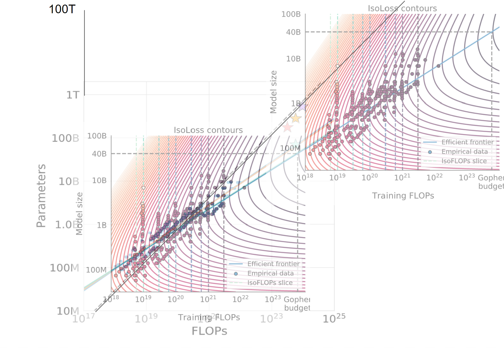
I took these graphs from the Chinchilla paper and then made them transparent and superimposed them on one another and then made a copy on the right to extend the line. And I drew some other lines to extend them.
Eyeballing this graph it looks like whatever performance we could achieve with 10^27 FLOPs under the Kaplan scaling laws, we can now achieve with 10^25 FLOPs. (!!!) This is a big deal if true. Am I reasoning incorrectly here?
If this is anywhere close to correct, then the distinction you mention between two methods of getting timelines -- "Assume it happens when we train a brain-sized model compute-optimally" vs. "assume it happens when we get to superhuman performance on this ensemble of benchmarks that we already have GPT trends for" becomes even more exciting and important than I thought! It's like, a huge huge crux, because it basically makes for a 4 OOM difference!
EDIT: To be clear, if this is true then I think I should update away from the second method, on the grounds that it predicts we are only about 1 OOM away and that seems implausible.
First I gotta say: I thought I knew the art of doing quick-and-dirty calculations, but holy crap, this methodology is quick-and-dirty-ier than I would ever have thought of. I'm impressed.
But I don't think it currently gets to right answer. One salient thing: it doesn't take into account Kaplan's "contradiction". I.e., Kaplan's laws already suggested that once we were using enough FLOP, we would have to scale data faster than we have to do in the short term. So when I made my extrapolations, I used a data-exponent that was larger than the one that's represented in that graph.
I now tried to do figure out the answer to this question using Chinchilla's loss curves and Kaplan's adjusted-for-contradiction loss curves, but I realised...
...that Chinchilla's "loss" and Kaplan's "loss" are pretty incomparable.
It's unsurprising that they're somewhat different (they might have used different datasets or something, when evaluating the loss), but I am surprised that Chinchilla's curves uses an additive term that predicts that loss will never go below 1.69. What happened with the claims that ideal text-prediction performance was like 0.7? (E.g. see here for me asking why gwern estimates 0.7, and gwern responding.)
Anyway, this makes it very non-obvious to me how to directly translate my benchmark extrapolations to a chinchilla context. Given that their "loss" is so different, I don't know what I could reasonably assume about the relationship between [benchmark performance as a function of chinchilla!loss] and [benchmark performance as a function of gpt-3!loss].
but I am surprised that Chinchilla's curves uses an additive term that predicts that loss will never go below 1.69. What happened with the claims that ideal text-prediction performance was like 0.7?
Apples & oranges, you're comparing different units. Comparing token perplexities is hard when the tokens (not to mention datasets) differ. Chinchilla isn't a character-level model but BPEs (well, they say SentencePiece which is more or less BPEs), and BPEs didn't even exist until the past decade so there will be no human estimates which are in BPE units (and I pity any subjects who are supposed to try to learn to predict the OA BPEs). If you want to handwave, BPEs are, I think, roughly equivalent to like 3 characters or bytes, so a bad upper bound on what ideal BPE loss would be 0.7*3=2.1, which is consistent with Chinchilla & Gopher hitting <2 BPE loss.
They do include bits-per-byte losses which vary widely but are indeed much closer to 0.7 than 1.69: https://arxiv.org/pdf/2203.15556.pdf#page=30 But no scaling laws on those you can grab an intrinsic entropy/irreducible loss from. Maybe there's some way to average over those bit-per-byte laws and translate the scaling law? The estimate would be pretty unstable, however: you can see how much the different corpuses vary, often by many times what the absolute remaining distance-to-true-human-loss must be.
You may be interested in this image. I would be grateful for critiques; maybe I'm thinking about it wrong?
Here's what the curves look like if you fit them to the PaLM data-points as well as the GPT-3 data-points.
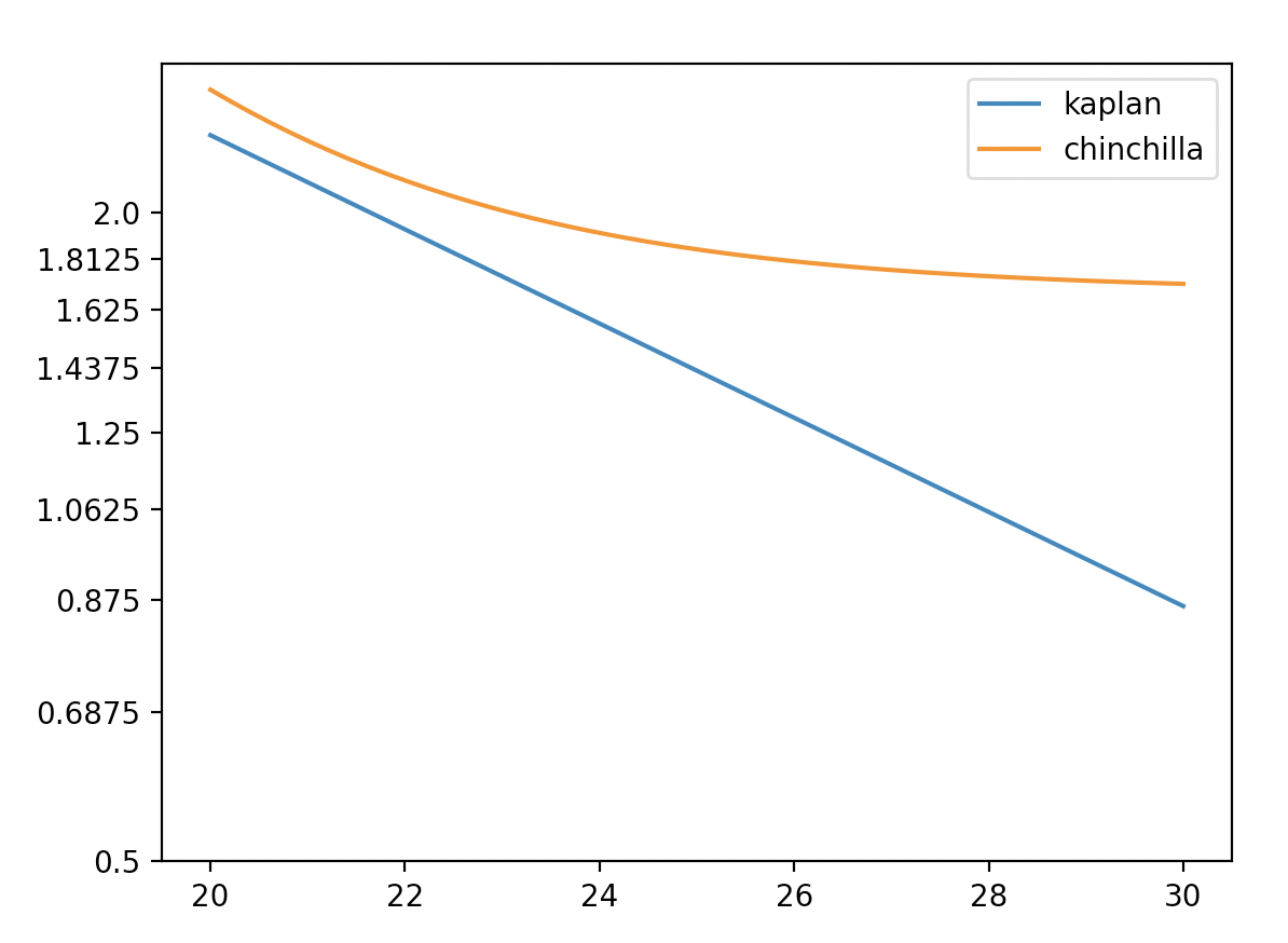
Keep in mind that this is still based on Kaplan scaling laws. The Chinchilla scaling laws would predict faster progress.
Linear:
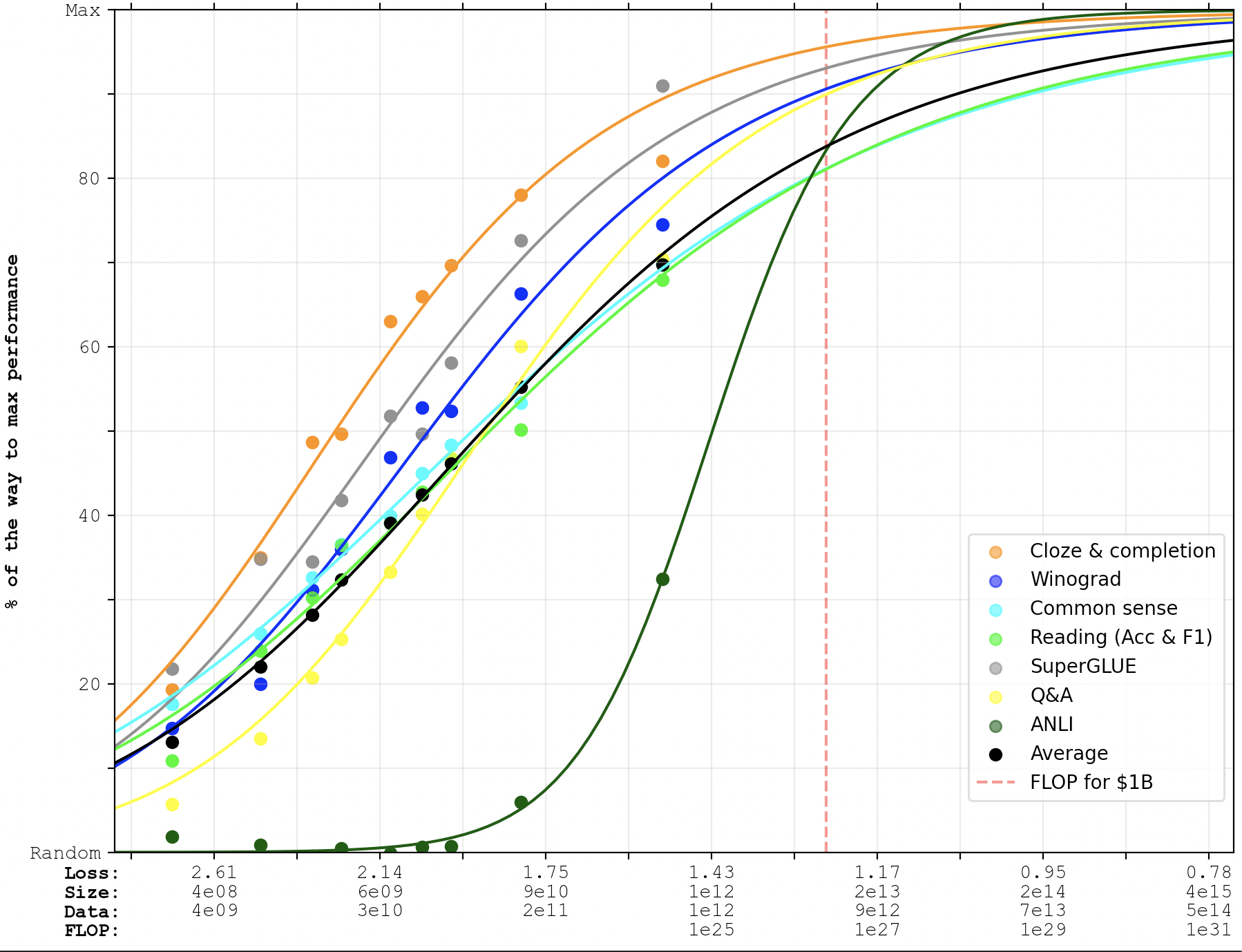
Logistic:
The Chinchilla scaling laws would predict faster progress.
(But we wouldn't observe that on these graphs because they weren't trained Chinchilla-style, of course.)
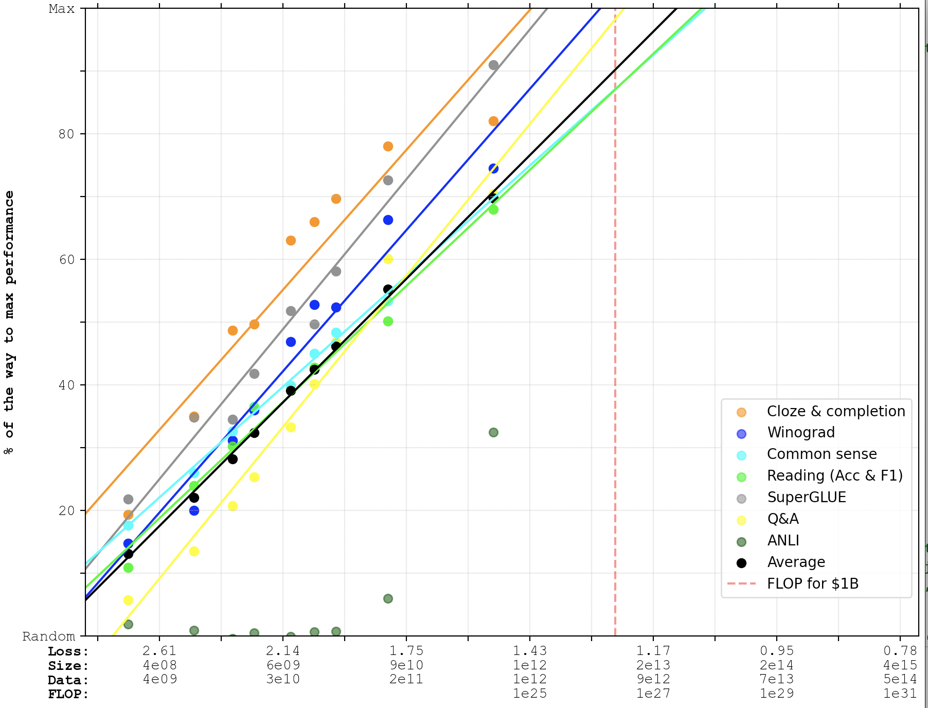
A bit more than a year ago, I wrote Extrapolating GPT-N performance, trying to predict how fast scaled-up models would improve on a few benchmarks. Google Research just released a paper reporting benchmark performance of PaLM: a 540B parameter model trained on 780B tokens. This post contains an updated version of one of the old graphs, where I've added PaLM's performance.
(Edit: I've made a further update here.)
You can read the original post for the full details, but as a quick explainer of how to read the graph:
Some reflections:
And a few caveats: