I am a bit confused how you deal with the problem of 0 eigenvalues in the Hessian. It seems like the reason that these 0 eigenvalues exist is because the basin volume is 0 as a subset of parameter space. My understanding right now of your fix is that you are adding along the diagonal to make the matrix full rank (and this quantity is coming from the regularization plus a small quantity). Geometrically, this seems like drawing a narrow ellipse around the subspace of which we are trying to estimate the volume.
But this doesn't seem natural to me, seems to me like the most important part of determining volume of these basins is the relative dimensionality. If there are two loss basins, but one has dimension greater than the other, the larger one dominates and becomes a lot more likely. If this is correct, we only care about the volume of basins that have the same number of dimensions. Thus, we can discard the dimensions with 0 eigenvalue and just apply the formula for the volume over the non-zero eigenvalues (but only for the basins with maximum rank hessians). This lets us directly compare the volume of these basins, and then treat the low dimensional basins as having 0 volume.
Does this make any sense?
The hessian is just a multi-dimensional second derivative, basically. So a zero eigenvalue is a direction along which the second derivative is zero (flatter-bottomed than a parabola).
So the problem is that estimating basin size this way will return spurious infinities, not zeros.
Thanks for your response! I'm not sure I communicated what I meant well, so let me be a bit more concrete. Suppose our loss is parabolic , where . This is like a 2d parabola (but it's convex hull / volume below a certain threshold is 3D). In 4D space, which is where the graph of this function lives and hence where I believe we are talking about basin volume, this has 0 volume. The hessian is the matrix:
This is conveniently already diagonal, and the 0 eigenvalue comes from the component , which is being ignored. My approach is to remove the 0-eigenspace, so we are working just in the subspace where the eigenvalues are positive, so we are left with just the matrix: , after which we can apply the formula given in the post:
If this determinant was 0 then dividing by 0 would get the spurious infinity (this is what you are talking about, right?). But if we remove the 0-eigenspace we are left with positive volume, and hence avoid this division by 0.
The loss is defined over all dimensions of parameter space, so is still a function of all 3 x's. You should think of it as . It's thickness in the direction is infinite, not zero.
Here's what a zero-determinant Hessian corresponds to:
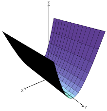
The basin here is not lower dimensional; it is just infinite in some dimension. The simplest way to fix this is to replace the infinity with some large value. Luckily, there is a fairly principled way to do this:
- Regularization / weight decay provides actual curvature, which should be added in to the loss, and doing this is the same as adding to the Hessian.
- The scale of the initialization distribution provides a natural scale for how much volume an infinite sweep should count as (very roughly, the volume only matters if it overlaps with the initialization distribution, and the distance of sweep for which this is true is on the order of , the standard deviation of the initialization).
So the is a fairly principled correction, and much better than just "throwing out" the other dimensions. "Throwing out" dimensions is unprincipled, dimensionally incorrect, numerically problematic, and should give worse results.
Note that this is equivalent to replacing "size 1/0" with "size 1". Issues with this become apparent if the scale of your system is much smaller or larger than 1. A better try might be to replace 0 with the average of the other eigenvalues, times a fudge factor. But still quite unprincipled - maybe better is to try to look at higher derivatives first or do nonlocal numerical estimation like described in the post.
Do you have thoughts on when there are two algorithms that aren’t “doing the same thing” that fall within the same loss basin?
It seems like there could be two substantially different algorithms which can be linearly interpolated between with no increase in loss. For example, the model is trained to classify fruit types and ripeness. One module finds the average color of a fruit (in an arbitrary basis), and another module uses this to calculate fruit type and ripeness. The basis in which color is expressed can be arbitrary, since the second module can compensate.
- Here, there are degrees of freedom in specifying the color basis and parameters can probably be eliminated, but it would be more interesting to see examples where two semantically different algorithms fall within the same basin without removable degrees of freedom, either because the Hessian has no zero eigenvalues, or because parameters cannot be removed despite the Hessian having a zero eigenvalue.
From this paper, "Theoretical work limited to ReLU-type activation functions, showed that in overparameterized networks, all global minima lie in a connected manifold (Freeman & Bruna, 2016; Nguyen, 2019)"
So for overparameterized nets, the answer is probably:
- There is only one solution manifold, so there are no separate basins. Every solution is connected.
- We can salvage the idea of "basin volume" as follows:
- In the dimensions perpendicular to the manifold, calculate the basin cross-section using the Hessian.
- In the dimensions parallel to the manifold, ask "how can I move before it stops being the 'same function'?". If we define "sameness" as "same behavior on the validation set",[1] then this means looking at the Jacobian of that behavior in the plane of the manifold.
- Multiply the two hypervolumes to get the hypervolume of our "basin segment" (very roughly, the region of the basin which drains to our specific model)
- ^
There are other "sameness" measures which look at the internals of the model; I will be proposing one in an upcoming post.
Thanks to Thomas Kwa for the question which prompted this post.
Note: This is mostly a primer / introductory reference, not a research post. However, the details should be interesting even to those familiar with the area.
When discussing “broad basins” in the loss landscape of a DNN, the Hessian of loss is often referenced. This post explains a simple theoretical approximation of basin volume which uses the Hessian of loss.[1]
Suppose our minimum has loss=0. Define the basin as the region of parameter space draining to our minimum where loss < threshold T.[2]
Simplest model
If all eigenvalues of the Hessian are positive and non trivial,[3] we can approximate the loss as a paraboloid centered on our minimum:
The vertical axis is loss, and the horizontal plane is parameter space. The shape of the basin in parameter space is the shadow of this paraboloid, which is an ellipsoid.
The principal directions of curvature of the paraboloid are given by the eigenvectors of the Hessian. The curvatures (second derivative) in each of those directions is given by the corresponding eigenvalue.
Radii of the ellipsoid: If we start at our minimum and walk away in a principal direction, the loss as a function of distance traveled is L(x)=12λix2, where λi is the Hessian eigenvalue for that direction. So given our loss threshold T, we will hit that threshold at a distance of x=√2Tλi. This is the radius of the loss-basin ellipsoid in that direction.
The volume of the ellipsoid is Vbasin=Vn∏i√2Tλi, where the constant Vn is the volume of the unit n-ball in n dimensions. Since the product of the eigenvalues is the determinant of the Hessian, we can write this as:
Vbasin=Vn(2T)n/2√det[Hessian]So the basin volume is inversely proportional to the square root of the determinant of the Hessian. Everything in the numerator is a constant, so only the determinant of the Hessian matters in this model.
The problem with this model is that the determinant of the Hessian is usually zero, due to zero eigenvalues.
Fixing the model
If we don't include a regularization term in the loss, the basin as we defined it earlier can actually be infinitely big (it's not just a problem with the paraboloid model). However, we don't really care about volume that is so far from the origin that it is never reached.
A somewhat principled way to fix the model is to look at volume weighted by the initialization distribution. This is easiest to work with if the initialization is Gaussian. To make the math tractable, we can replace our ellipsoid with a "fuzzy ellipsoid" -- i.e. a multivariate Gaussian. Now we just have to integrate the product of two Gaussians, which should be easy. There are also somewhat principled reasons for using a "fuzzy ellipsoid", which I won't explain here.
However, this is only somewhat principled; if you think about it further, it starts to become unclear: Should we use the initialization Gaussian, or one based on the expected final L2 norm? What about cases where the norm peaks in the middle of training, and is smaller at the start and finish?
If we have an L2 regularization term in the loss, then the infinite volume problem usually goes away; the L2 term makes all the eigenvalues positive, so the formula is fine. If we have weight decay, we can interpret this as L2 regularization and add it to the loss.
For a relatively simple approximation, I recommend the formula:
Vbasin=Vn(2T)n/2√det[Hessian(Loss) + (λ+c)In]Where:
Estimation in practice
If the DNN of interest is large (>10k params for instance), the Hessian becomes very unwieldy.[4] Luckily, it is possible to efficiently estimate the quantity det[Hessian(Loss) + (λ+c)In] without ever computing the Hessian.
One correct[5] method of doing this is to get the eigenvalue spectrum of the Hessian using stochastic Lanczos quadrature.[6] Then shift the spectrum up by λ+c and estimate the product.
Roasting the literature a bit
The "easy way out" is to use the trace of the Hessian instead of the determinant. This is extremely easy to estimate: Just sample the second derivative in random directions, and the average value is proportional to the trace. The problem is that the trace is simply the wrong measure, and is probably a somewhat poor proxy for the determinant.
Most (all?) of the flatness and volume measures I have seen in the literature are actually tracking the trace. There is one (Keskar et. al.)[7] which seems to be correcting in the wrong direction (increasing the influence of large eigenvalues relative to the trace, when it should be doing the opposite).[8] There is another which samples ellipsoid radius in random directions and calculates the volume of an ellipsoid slice in that direction (which is proportional to rn). While this is technically an unbiased estimator for finite ellipsoids, it has two problems in practice:[9]
Information theory
How many bits does it take to specify (locate) a loss basin?
The simplest answer is −log2(V), where V is the initialization-weighted volume of the basin. The weighting is done such that it integrates to 1.
Note that this model is nowhere close to perfect, and also isn’t computationally tractable for large networks without further tricks/approximations.
Having a threshold isn't necessarily desirable or standard, but it makes it easier to model.
This condition basically never happens for DNNs; we'll see how to fix this in the next section.
I think explicitly calculating the eigenvalues and eigenvectors is O(n3)
This only works well if (λ+c) is significantly larger than the resolution of the stochastic Lanczos quadrature.
Warning: The math is very hard to understand. I think library implementations exist online; I have not used them though. If you try implementing it yourself, it will probably be a massive pain.
This paper is widely cited and generally very good.
The determinant is a product, so it is more sensitive to small eigenvalues than the trace.
I have confirmed with simulations that it is flawed for very large n. Doing the equivalent of our (λ+c)In correction fixes the first issue but not the second.
Summary of the first two sections: You can approximate the loss as a paraboloid, which gives you an ellipsoid as the basin. The eigenvalues of the Hessian of loss give you the curvatures. The volume of the ellipsoid is proportional to 1√det[Hessian] (recall that determinant = product of eigenvalues). This doesn't actually work because the eigenvalues can be zero. You can fix this by adding a constant to every eigenvalue.