This is a more technical followup to the last post, putting precise bounds on when regressional Goodhart leads to failure or not. We'll first show conditions under which optimization for a proxy fails, and then some conditions under which it succeeds. (The second proof will be substantially easier.)
Related work
In addition to the related work sections of the previous post, this post makes reference to the textbook An Introduction to Heavy-Tailed and Subexponential Distributions, by Foss et al. Many similar results about random variables are present in the textbook, though we haven't seen this posts's results elsewhere in the literature before. We mostly adopt their notation here, and cite a few helpful lemmas.
Main result: Conditions for catastrophic Goodhart
Suppose that X and V are independent real-valued random variables. We're going to show, roughly, that if
X is subexponential (a slightly stronger property than being heavy-tailed).
V has lighter tails than X by more than a linear factor, meaning that the ratio of the tails of V and the tails of X grows superlinearly.[1]
then limt→∞E[V|X+V≥t]=E[V].
Less formally, we're saying something like "if it requires relatively little selection pressure on X to get more of X and asymptotically more selection pressure on V to get more of V, then applying very strong optimization towards X+V will not get you even a little bit of optimization towards V - all the optimization power will go towards X."
Proof sketch and intuitions
The conditional expectation E[V|X+V>t] is given by ∫∞−∞vfV(v)Pr(X>t−v)∫∞−∞fV(v)Pr(X>t−v),[2] and we divide the integral in the numerator into 4 regions, showing that each region's effect on the conditional expectation of V is similar to that of the corresponding region in the unconditional expectation E[V].
The regions are defined in terms of a slow-growing function h(t):R→R≥0 such that the fiddly bounds on different pieces of the proof work out. Roughly, we want it to go to infinity so that |V| is likely to be less than h(t) in the limit, but grow slowly enough that the shape of V's distribution within the interval [−h(t),h(t)] doesn't change much after conditioning.
In the table below, we abbreviate the condition X+V>t as c.
Region
Why its effect on E[V|c] is small
Explanation
r1=(−∞,−h(t)]
P[V∈r1|c] is too low
In this region, |V|>h(t) and X>t+h(t), both of which are unlikely.
r2=(−h(t),h(t))
E[V|V∈r2,c]≈E[V|V∈r2]
The tail distribution of X is too flat to change the shape of V's distribution within this region.
r3=[h(t),t−h(t)]
P[V∈r3|c] is low, and V<t.
There are increasing returns to each bit of optimization for X, so it's unlikely that both X and V have moderate values.[3]
r4=(t−h(t),∞)
P[V∈r4|c] is too low
X is heavier-tailed than V, so the condition that V>t−h(t) is much less likely than X>t−h(t) in r2.
Here's a diagram showing the region boundaries at −h(t), h(t), and t−h(t) in an example where t=25 and h(t)=4, along with a negative log plot of the relevant distribution:
Note that up to a constant vertical shift of normalization, the green curve is the pointwise sum of the blue and orange curves.
Full proof
To be more precise, we're going to make the following definitions and assumptions:
Let fV(v) be the PDF of V at the value v. We assume for convenience that fV exists, is integrable, etc, though we suspect that this isn't necessary, and that one could work through a similar proof just referring to the tails of V. We won't make this assumption for X.
Let FX(x)=Pr(X≤x) and ¯FX(x)=Pr(X>x), similarly for FV and ¯FV.
Assume V has a finite mean: ∫∞−∞vfV(v)dv converges absolutely.
Formally, this means that limx→∞Pr(X1+X2>x)Pr(X>x)=2.
This happens roughly whenever X has tails that are heavier than e−cx for any c and is reasonably well-behaved; counterexamples to the claim "long-tailed implies subexponential" exist, but they're nontrivial to exhibit.
Examples of subexponential distributions include log-normal distributions, anything that decays like a power law, the Pareto distribution, and distributions with tails asymptotic to e−xa for any 0<a<1.
We require for V that its tail function is substantially lighter than X's, namely thatlimt→∞tp¯FV(t)¯FX(t)=0 for some p>1.[1]
This implies that ¯FV(t)=O(¯FX(t)/t).
With all that out of the way, we can move on to the proof.
The unnormalized PDF of V conditioned on X+V≥t is given by fV(v)¯FX(t−v). Its expectation is given by ∫∞−∞vfV(v)¯FX(t−v)∫∞−∞fV(v)¯FX(t−v).
Meanwhile, the unconditional expectation of V is given by ∫∞−∞vfV(v).
We'd like to show that these two expectations are equal in the limit for large t. To do this, we'll introduce Q(v)=¯FX(t−v)¯FX(t). (More pedantically, this should really be Qt(v), which we'll occasionally use where it's helpful to remember that this is a function of t.)
For a given value of t, Q(v) is just a scaled version of ¯FX(t−v), so the conditional expectation of V is given by ∫∞−∞vfV(v)Q(v)∫∞−∞fV(v)Q(v). But because Q(0)=1, the numerator and denominator of this fraction are (for small v) close to the unconditional expectation and 1, respectively.
We'll aim to show that for all ϵ>0, we have for sufficiently large t that ∣∣∫∞−∞vfV(v)Qt(v)−∫∞−∞vfV(v)∣∣<ϵ and ∫∞−∞fV(v)Qt(v)∈[1−ϵ,1+ϵ], which implies (exercise) that the two expectations have limiting difference zero. But first we need some lemmas.
Lemmas
Lemma 1: There is h(t) depending on FX such that:
(a) limx→∞h(t)=∞
(b) limt→∞t−h(t)=∞
(c) limt→∞¯FX(t−h(t))¯FX(t)=1
(d) limt→∞sup|v|≤h(t)|Q(v,t)−1|=0.
Proof: Lemma 2.19 from Foss implies that if X is long-tailed (which it is, because subexponential implies long-tailed), then there is h(t) such that condition (a) holds and ¯FX is h-insensitive; by Proposition 2.20 we can take h such that h(t)≤t/2 for sufficiently large t, implying condition (b). Conditions (c) and (d) follow from being h-insensitive.
Lemma 2: Suppose that FX is whole-line subexponential and h is chosen as in Lemma 1. Also suppose that ¯FV(t)=O(¯FX(t)/t). Then Pr[X+V>t,V>h(t),X>h(t)]=o(¯FX(t)/t).
Proof: This is a slight variation on lemma 3.8 from [1], and follows from the proof of Lemma 2.37. Lemma 2.37 states that
where X,X′∼FX. Multiplying by t, we have tP{X+V>t,X>h(t),V>h(t)}≤supz>h(t)t¯FV(z)¯FX(z)P{X+X′>t,X>h(t),X′>h(t)},
and because h(t)→∞ as t→∞ and ¯FV(t)=O(¯FX(t)/t), we can say that for some c<∞, limt→∞supz>h(t)t¯FV(z)¯FX(z)<c. Therefore for sufficiently large tP{X+V>t,X>h(t),V>h(t)}≤ctP{X+X′>t,X>h(t),X′>h(t)}.
By Theorem 3.6, P{X+X′>t,X>h(t),X′>h(t)} is o(¯FX(t)), so the LHS is o(¯FX(t)/t) as desired.
Bounds on the numerator
We want to show, for arbitrary ϵ>0, that ∣∣∫∞−∞vfV(v)Q(v)−∫∞−∞vfV(v)∣∣<ϵ in the limit as t→∞. Since
it will suffice to show that the latter quantity is less than ϵ for large t.
We're going to show that ∫∞−∞|v|⋅fV(v)⋅|Q(v)−1| is small by showing that the integral gets arbitrarily small on each of four pieces: (−∞,−h(t)], (−h(t),h(t)), [h(t),t−h(t)], and (t−h(t),∞).
We'll handle these case by case (they'll get monotonically trickier).
Region 1: (−∞,−h(t)]
Since ∫∞−∞vfV(v) is absolutely convergent, for sufficiently large t we will have∫−h(t)−∞|v|fV(v)<ϵ, since h(t) goes to infinity by Lemma 1(a).
Since Q(v) is monotonically increasing and Q(0)=1, we know that in this interval |Q(v)−1|=1−Q(v).
By lemma 1(d), h is such that for sufficiently large t, |Q(v)−1|<ϵ∫∞−∞|v|fV(v) on the interval [−h(t),h(t)]. (Note that the value of this upper bound depends only on V and ϵ, not on t or h.) So we have
it would suffice to show that the latter expression becomes less than ϵ for large t, or equivalently that ∫t−h(t)h(t)fV(v)¯FX(t−v)=o(¯FX(t)t) .
The LHS in this expression is the unconditional probability that X+V>t and h(t)<V<t−h(t), but this event implies X+V>t,V>h(t), and X>h(t). So we can write
∫t−h(t)h(t)fV(v)¯FX(t−v)=Pr[X+V>t,h(t)<V<t−h(t)]
<Pr[X+V>t,V>h(t),X>h(t)]=o(¯FX(t)/t) by Lemma 2.
Region 4: (t−h(t),∞)
For the fourth part, we'd like to show that ∫∞t−h(t)vfV(v)Q(v)→0 for large t.
Since Q(v)=¯FX(t−v)¯FX(t)<1¯FX(t), it would suffice to show ∫∞t−h(t)vfV(v)=o(¯FX(t)). But note that since limt→∞¯FX(t−h(t))¯FX(t)=1 by Lemma 1(c), this is equivalent to ∫∞t−h(t)vfV(v)=o(¯FX(t−h(t))), which (by Lemma 1(b)) is equivalent to ∫∞tvfV(v)=o(¯FX(t)).
Note that ∫∞tvfV(v)=t∫∞tfV(v)+∫∞t(v−t)fV(v)=t¯FV(t)+∫∞t¯FV(v), so it will suffice to show that both terms in this sum are o(¯FX(t)).
The first term t¯FV(t) is o(¯FX(t)) because we assumed limt→∞tp¯FV(t)¯FX(t)=0 for some p>1.
For the second term, we have for the same reason∫∞t¯FV(v)<∫∞t¯FX(v)vp=¯FX(t)∫∞tv−p=t1−pp−1¯FX(t)=o(¯FX(t)).
This completes the bounds on the numerator.
Bounds on the denominator
For the denominator, we want to show that limt→∞∫∞−∞fV(v)Qt(v)=1=∫∞−∞fV(v), so it'll suffice to show |∫∞−∞fV(v)(Qt(v)−1)|=o(1) as t→∞.
Again, we'll break up this integral into pieces, though they'll be more straightforward than last time. We'll look at (−∞,−h(t)), [−h(t),h(t)], and (h(t),∞).
But for sufficiently large t we have h(t)>1, so we obtain ∫∞h(t)fV(v)Q(v)<∫∞h(t)vfV(v)Q(v)<∫∞−∞vfV(v)Q(v)=o(1) by the results of the previous section.
This completes the proof!
Light tails imply V
Conversely, here's a case where we do get arbitrarily high E[V|X+V≥t] for large t. This generalizes a consequence of the lemma from Appendix A of Scaling Laws for Reward Model Overoptimization (Gao et al., 2022), which shows this result in the case where X is either bounded or normally distributed.
Suppose that X satisfies the property that limt→∞¯FX(t+1)¯FX(t)=0.[4] This implies that X has tails that are dominated by e−cx for any c, though it's a slightly stronger claim because it requires that X not be too "jumpy" in the decay of its tails.[5]
We'll show that for any V with a finite mean which has no upper bound, limt→∞E[V|X+V>t]=∞.
In particular we'll show that for any c, limt→∞E[V|X+V>t]≥c.
Proof
Let Pr(V>c+1)=p>0, which exists by our assumption that V is unbounded.
Let E[V|V<c]=q. (If this is undefined because the conditional has probability 0, we'll have the desired result anyway since then V would always be at least c.)
Observe that for all t, E[V|V<c,X+V>t]≥q (assuming it is defined), because we're conditioning (V|V<c) on an event which is more likely for larger v (since X and V are independent).
First, let's see that limt→∞P(V<c|X+V≥t)P(V>c+1|X+V≥t)=0. This ratio of probabilities is equal to
which, by our assumption that limt→∞¯FX(t+1)¯FX(t)=0, will get arbitrarily small as t increases for any positive p.
Now, consider E[V|X+V≥t]. We can break this up as the sum across outcomes Z of E[V|Z,X+V≥t]⋅Pr(Z|X+V≥t) for the three disjoint outcomes V<c, c≤V≤c+1, and V>c+1. Note that we can lower bound these expectations by q,c,c+1 respectively. But then once t is large enough that Pr(V<c|X+V≥t)Pr(V>c+1|X+V≥t)<1c−q, this weighted sum of conditional expectations will add to more than c (exercise).
Answers to exercises from last post
Show that when X and V are independent and t∈R, E[V|X+V>t]≥E[V]. Conclude that limt→∞E[V|X+V>t]≥E[V]. This means that given independence, optimization always produces a plan that is no worse than random.
Proof: Fixing a value of t, we have for all x∈R thatE(V|X+V>t,X=x)=E(V|V>t−x)≥E(V). Since the conditional expectation after seeing any particular value of X is at least E(V), this will be true when averaged across all x proportional to their frequency in the distribution of X. This means that E[X+V>t]≥E(V) for all t, so the inequality also holds in the limit.
When independence is violated, an optimized plan can be worse than random, even if your evaluator is unbiased. Construct a joint distribution fVX for X and V such that E[X]=0, E[V]=0, and E[X|V=v]=0 for any v∈R, but limt→∞E[V|X+V>t]=−∞.
Solution: Suppose that V is distributed with a PDF equal to 0.5e−|v|, and the conditional distribution of X is given by
(X|V=v)={0v≥0Coinflip()⋅(v2−v)v<0 where Coinflip() is a random variable that is equal to ±1 with 50/50 odds. The two-dimensional heatmap looks like this: Now, conditioning on X+V≥t with t>0, we have one of two outcomes: either V≥t, or V≤−√t and Coinflip()=1. The first case has an unconditional probability of 0.5e−t, and a conditional expectation of E[V|V≥t]=∫∞t0.5ve−vdv∫∞t0.5e−vdv=0.5(t+1)e−t0.5e−t=t+1. The second case has an unconditional probability of 0.25e−√t, and a conditional expectation of at most −√t since all values of v in the second case are at most that large. So, abbreviating these two cases as A and B respectively, the overall conditional expectation is given by E[V|X+V≥t]=E[V|A]Pr(A)+E[V|B]Pr(B)Pr(A)+Pr(B)≤(t+1)0.5e−t−0.25e−√t√t0.5e−t+0.25e−√t =(2t+2)−e√t√t2+e√t≤(2t+2)−e√t√te√t=(2t+2)e√t−√t=o(1)−√t→−∞ as desired.
This sort of strategy works for any fixed distribution of V, so long as the distribution is not bounded below and has finite mean; we can replace v2−v with some sufficiently fast-growing function to get a zero-mean conditional X distribution that behaves the same.
For a followup exercise, construct an example of this behavior even when all conditional X distributions have variance at most 1.
The diagrams in the previous post show visually that when X and V are both heavy-tailed and t is large, most of the probability mass has X≈0, V≈t or vice versa.
This proof will actually go through if we just have limt→∞¯FX(t+k)¯FX(t)=0 for any constant k>0, which is a slightly weaker condition (just replace 1 with k in the proof as necessary). For instance, X could have probability en! of being equal to 100n for n=0,1,2,3,…, which would satisfy this condition for k=101 but not k=1.
If X has really jumpy tails, the limit of the mean of the conditional distribution may not exist. Exercise: what goes wrong when X has a 23n probability of being equal to 2n for n=1,2,3,… and V is a standard normal distribution?
This is a more technical followup to the last post, putting precise bounds on when regressional Goodhart leads to failure or not. We'll first show conditions under which optimization for a proxy fails, and then some conditions under which it succeeds. (The second proof will be substantially easier.)
Related work
In addition to the related work sections of the previous post, this post makes reference to the textbook An Introduction to Heavy-Tailed and Subexponential Distributions, by Foss et al. Many similar results about random variables are present in the textbook, though we haven't seen this posts's results elsewhere in the literature before. We mostly adopt their notation here, and cite a few helpful lemmas.
Main result: Conditions for catastrophic Goodhart
Suppose that X and V are independent real-valued random variables. We're going to show, roughly, that if
then limt→∞E[V|X+V≥t]=E[V].
Less formally, we're saying something like "if it requires relatively little selection pressure on X to get more of X and asymptotically more selection pressure on V to get more of V, then applying very strong optimization towards X+V will not get you even a little bit of optimization towards V - all the optimization power will go towards X."
Proof sketch and intuitions
The conditional expectation E[V|X+V>t] is given by ∫∞−∞vfV(v)Pr(X>t−v)∫∞−∞fV(v)Pr(X>t−v),[2] and we divide the integral in the numerator into 4 regions, showing that each region's effect on the conditional expectation of V is similar to that of the corresponding region in the unconditional expectation E[V].
The regions are defined in terms of a slow-growing function h(t):R→R≥0 such that the fiddly bounds on different pieces of the proof work out. Roughly, we want it to go to infinity so that |V| is likely to be less than h(t) in the limit, but grow slowly enough that the shape of V's distribution within the interval [−h(t),h(t)] doesn't change much after conditioning.
In the table below, we abbreviate the condition X+V>t as c.
Here's a diagram showing the region boundaries at −h(t), h(t), and t−h(t) in an example where t=25 and h(t)=4, along with a negative log plot of the relevant distribution:
Note that up to a constant vertical shift of normalization, the green curve is the pointwise sum of the blue and orange curves.
Full proof
To be more precise, we're going to make the following definitions and assumptions:
With all that out of the way, we can move on to the proof.
The unnormalized PDF of V conditioned on X+V≥t is given by fV(v)¯FX(t−v). Its expectation is given by ∫∞−∞vfV(v)¯FX(t−v)∫∞−∞fV(v)¯FX(t−v).
Meanwhile, the unconditional expectation of V is given by ∫∞−∞vfV(v).
We'd like to show that these two expectations are equal in the limit for large t. To do this, we'll introduce Q(v)=¯FX(t−v)¯FX(t). (More pedantically, this should really be Qt(v), which we'll occasionally use where it's helpful to remember that this is a function of t.)
For a given value of t, Q(v) is just a scaled version of ¯FX(t−v), so the conditional expectation of V is given by ∫∞−∞vfV(v)Q(v)∫∞−∞fV(v)Q(v). But because Q(0)=1, the numerator and denominator of this fraction are (for small v) close to the unconditional expectation and 1, respectively.
We'll aim to show that for all ϵ>0, we have for sufficiently large t that ∣∣∫∞−∞vfV(v)Qt(v)−∫∞−∞vfV(v)∣∣<ϵ and ∫∞−∞fV(v)Qt(v)∈[1−ϵ,1+ϵ], which implies (exercise) that the two expectations have limiting difference zero. But first we need some lemmas.
Lemmas
Lemma 1: There is h(t) depending on FX such that:
Proof: Lemma 2.19 from Foss implies that if X is long-tailed (which it is, because subexponential implies long-tailed), then there is h(t) such that condition (a) holds and ¯FX is h-insensitive; by Proposition 2.20 we can take h such that h(t)≤t/2 for sufficiently large t, implying condition (b). Conditions (c) and (d) follow from being h-insensitive.
Lemma 2: Suppose that FX is whole-line subexponential and h is chosen as in Lemma 1. Also suppose that ¯FV(t)=O(¯FX(t)/t). Then Pr[X+V>t, V>h(t), X>h(t)]=o(¯FX(t)/t).
Proof: This is a slight variation on lemma 3.8 from [1], and follows from the proof of Lemma 2.37. Lemma 2.37 states that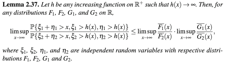
but it is actually proved that
P{ξ1+η1>x,ξ1>h(x),η1>h(x)}≤supz>h(x)¯¯¯¯¯¯F1(z)¯¯¯¯¯¯F2(z)⋅supz>h(x)¯¯¯¯¯¯G1(z)¯¯¯¯¯¯G2(z)⋅P{ξ2+η2>x,ξ2>h(x),η2>h(x)}.
If we let F1=FV,F2=G1=G2=FX, then we get
P{X+V>t,X>h(t),V>h(t)}≤supz>h(t)¯FV(z)¯FX(z)supz>h(t)¯FX(z)¯FX(z)P{X+X′>t,X>h(t),X′>h(t)}=supz>h(t)¯FV(z)¯FX(z)P{X+X′>t,X>h(t),X′>h(t)}
where X,X′∼FX. Multiplying by t, we have tP{X+V>t,X>h(t),V>h(t)}≤supz>h(t)t¯FV(z)¯FX(z)P{X+X′>t,X>h(t),X′>h(t)},
and because h(t)→∞ as t→∞ and ¯FV(t)=O(¯FX(t)/t), we can say that for some c<∞, limt→∞supz>h(t)t¯FV(z)¯FX(z)<c. Therefore for sufficiently large tP{X+V>t,X>h(t),V>h(t)}≤ctP{X+X′>t,X>h(t),X′>h(t)}.
By Theorem 3.6, P{X+X′>t,X>h(t),X′>h(t)} is o(¯FX(t)), so the LHS is o(¯FX(t)/t) as desired.
Bounds on the numerator
We want to show, for arbitrary ϵ>0, that ∣∣∫∞−∞vfV(v)Q(v)−∫∞−∞vfV(v)∣∣<ϵ in the limit as t→∞. Since
∣∣∫∞−∞vfV(v)Q(v)−∫∞−∞vfV(v)∣∣≤∫∞−∞|vfV(v)(Q(v)−1)|=∫∞−∞|v|⋅fV(v)⋅|Q(v)−1|
it will suffice to show that the latter quantity is less than ϵ for large t.
We're going to show that ∫∞−∞|v|⋅fV(v)⋅|Q(v)−1| is small by showing that the integral gets arbitrarily small on each of four pieces: (−∞,−h(t)], (−h(t),h(t)), [h(t),t−h(t)], and (t−h(t),∞).
We'll handle these case by case (they'll get monotonically trickier).
Region 1: (−∞,−h(t)]
Since ∫∞−∞vfV(v) is absolutely convergent, for sufficiently large t we will have∫−h(t)−∞|v|fV(v)<ϵ, since h(t) goes to infinity by Lemma 1(a).
Since Q(v) is monotonically increasing and Q(0)=1, we know that in this interval |Q(v)−1|=1−Q(v).
So we have
∫−h(t)−∞|v|⋅fV(v)⋅|Q(v)−1|=∫−h(t)−∞|v|fV(v)(1−Q(v))<∫−h(t)−∞|v|fV(v)<ϵ
as desired.
Region 2: (−h(t),h(t))
By lemma 1(d), h is such that for sufficiently large t, |Q(v)−1|<ϵ∫∞−∞|v|fV(v) on the interval [−h(t),h(t)]. (Note that the value of this upper bound depends only on V and ϵ, not on t or h.) So we have
∫h(t)−h(t)|v|fV(v)|Q(v)−1|<ϵ∫∞−∞|v|fV(v)∫h(t)−h(t)|v|fV(v)<ϵ∫∞−∞|v|fV(v)∫∞−∞|v|fV(v)=ϵ.
Region 3: [h(t),t−h(t)]
For the third part, we'd like to show that ∫t−h(t)h(t)vfV(v)(Q(v)−1)<ϵ. Since
∫t−h(t)h(t)vfV(v)(Q(v)−1)<∫t−h(t)h(t)tfV(v)Q(v)=t¯FX(t)∫t−h(t)h(t)fV(v)¯FX(t−v)
it would suffice to show that the latter expression becomes less than ϵ for large t, or equivalently that ∫t−h(t)h(t)fV(v)¯FX(t−v)=o(¯FX(t)t) .
The LHS in this expression is the unconditional probability that X+V>t and h(t)<V<t−h(t), but this event implies X+V>t,V>h(t), and X>h(t). So we can write
∫t−h(t)h(t)fV(v)¯FX(t−v)=Pr[X+V>t, h(t)<V<t−h(t)]
<Pr[X+V>t, V>h(t), X>h(t)]=o(¯FX(t)/t) by Lemma 2.
Region 4: (t−h(t),∞)
For the fourth part, we'd like to show that ∫∞t−h(t)vfV(v)Q(v)→0 for large t.
Since Q(v)=¯FX(t−v)¯FX(t)<1¯FX(t), it would suffice to show ∫∞t−h(t)vfV(v)=o(¯FX(t)). But note that since limt→∞¯FX(t−h(t))¯FX(t)=1 by Lemma 1(c), this is equivalent to ∫∞t−h(t)vfV(v)=o(¯FX(t−h(t))), which (by Lemma 1(b)) is equivalent to ∫∞tvfV(v)=o(¯FX(t)).
Note that ∫∞tvfV(v)=t∫∞tfV(v)+∫∞t(v−t)fV(v)=t¯FV(t)+∫∞t¯FV(v), so it will suffice to show that both terms in this sum are o(¯FX(t)).
The first term t¯FV(t) is o(¯FX(t)) because we assumed limt→∞tp¯FV(t)¯FX(t)=0 for some p>1.
For the second term, we have for the same reason∫∞t¯FV(v)<∫∞t¯FX(v)vp=¯FX(t)∫∞tv−p=t1−pp−1¯FX(t)=o(¯FX(t)).
This completes the bounds on the numerator.
Bounds on the denominator
For the denominator, we want to show that limt→∞∫∞−∞fV(v)Qt(v)=1=∫∞−∞fV(v), so it'll suffice to show |∫∞−∞fV(v)(Qt(v)−1)|=o(1) as t→∞.
Again, we'll break up this integral into pieces, though they'll be more straightforward than last time. We'll look at (−∞,−h(t)), [−h(t),h(t)], and (h(t),∞).
≤sup|v|≤h(t)|Q(v,t)−1|∫h(t)−h(t)fV(v)≤sup|v|≤h(t)|Q(v,t)−1|
∫∞h(t)fV(v)Q(v)<∫∞h(t)vfV(v)Q(v)<∫∞−∞vfV(v)Q(v)=o(1)
by the results of the previous section.
This completes the proof!
Light tails imply V
Conversely, here's a case where we do get arbitrarily high E[V|X+V≥t] for large t. This generalizes a consequence of the lemma from Appendix A of Scaling Laws for Reward Model Overoptimization (Gao et al., 2022), which shows this result in the case where X is either bounded or normally distributed.
Suppose that X satisfies the property that limt→∞¯FX(t+1)¯FX(t)=0.[4] This implies that X has tails that are dominated by e−cx for any c, though it's a slightly stronger claim because it requires that X not be too "jumpy" in the decay of its tails.[5]
We'll show that for any V with a finite mean which has no upper bound, limt→∞E[V|X+V>t]=∞.
In particular we'll show that for any c, limt→∞E[V|X+V>t]≥c.
Proof
Let Pr(V>c+1)=p>0, which exists by our assumption that V is unbounded.
Let E[V|V<c]=q. (If this is undefined because the conditional has probability 0, we'll have the desired result anyway since then V would always be at least c.)
Observe that for all t, E[V|V<c,X+V>t]≥q (assuming it is defined), because we're conditioning (V|V<c) on an event which is more likely for larger v (since X and V are independent).
First, let's see that limt→∞P(V<c|X+V≥t)P(V>c+1|X+V≥t)=0. This ratio of probabilities is equal to
∫c−∞fV(v)¯FX(t−v)∫∞c+1fV(v)¯FX(t−v)≤∫c−∞fV(v)¯FX(t−c)∫∞c+1fV(v)¯FX(t−c−1)=¯FX(t−c)¯FX(t−c−1)⋅∫c−∞fV(v)∫∞c+1fV(v)
=¯FX(t−c)¯FX(t−c−1)⋅Pr(V<c)Pr(V>c+1)≤¯FX(t−c)¯FX(t−c−1)⋅1p
which, by our assumption that limt→∞¯FX(t+1)¯FX(t)=0, will get arbitrarily small as t increases for any positive p.
Now, consider E[V|X+V≥t]. We can break this up as the sum across outcomes Z of E[V|Z,X+V≥t]⋅Pr(Z|X+V≥t) for the three disjoint outcomes V<c, c≤V≤c+1, and V>c+1. Note that we can lower bound these expectations by q,c,c+1 respectively. But then once t is large enough that Pr(V<c|X+V≥t)Pr(V>c+1|X+V≥t)<1c−q, this weighted sum of conditional expectations will add to more than c (exercise).
Answers to exercises from last post
Proof: Fixing a value of t, we have for all x∈R thatE(V|X+V>t,X=x)=E(V|V>t−x)≥E(V). Since the conditional expectation after seeing any particular value of X is at least E(V), this will be true when averaged across all x proportional to their frequency in the distribution of X. This means that E[X+V>t]≥E(V) for all t, so the inequality also holds in the limit.
Solution: Suppose that V is distributed with a PDF equal to 0.5e−|v|, and the conditional distribution of X is given by
(X|V=v)={0v≥0Coinflip()⋅(v2−v)v<0
where Coinflip() is a random variable that is equal to ±1 with 50/50 odds. The two-dimensional heatmap looks like this:
Now, conditioning on X+V≥t with t>0, we have one of two outcomes: either V≥t, or V≤−√t and Coinflip()=1.
The first case has an unconditional probability of 0.5e−t, and a conditional expectation of E[V|V≥t]=∫∞t0.5ve−vdv∫∞t0.5e−vdv=0.5(t+1)e−t0.5e−t=t+1.
The second case has an unconditional probability of 0.25e−√t, and a conditional expectation of at most −√t since all values of v in the second case are at most that large.
So, abbreviating these two cases as A and B respectively, the overall conditional expectation is given by
E[V|X+V≥t]=E[V|A]Pr(A)+E[V|B]Pr(B)Pr(A)+Pr(B)≤(t+1)0.5e−t−0.25e−√t√t0.5e−t+0.25e−√t
=(2t+2)−e√t√t2+e√t≤(2t+2)−e√t√te√t=(2t+2)e√t−√t=o(1)−√t→−∞
as desired.
This sort of strategy works for any fixed distribution of V, so long as the distribution is not bounded below and has finite mean; we can replace v2−v with some sufficiently fast-growing function to get a zero-mean conditional X distribution that behaves the same.
For a followup exercise, construct an example of this behavior even when all conditional X distributions have variance at most 1.
We actually just need ∫∞t¯FV(v)∈o(¯FX(t)), so we can have e.g. ¯FV(v)=FX(v)vlog2(v).
We'll generally omit dx and dv terms in the interests of compactness and laziness; the implied differentials should be pretty clear.
The diagrams in the previous post show visually that when X and V are both heavy-tailed and t is large, most of the probability mass has X≈0, V≈t or vice versa.
This proof will actually go through if we just have limt→∞¯FX(t+k)¯FX(t)=0 for any constant k>0, which is a slightly weaker condition (just replace 1 with k in the proof as necessary). For instance, X could have probability en! of being equal to 100n for n=0,1,2,3,…, which would satisfy this condition for k=101 but not k=1.
If X has really jumpy tails, the limit of the mean of the conditional distribution may not exist. Exercise: what goes wrong when X has a 23n probability of being equal to 2n for n=1,2,3,… and V is a standard normal distribution?